No. 453: June Employment and Unemployment, Money Supply M3
COMMENTARY NUMBER 453
June Employment and Unemployment, Money Supply M3
July 6, 2012
__________
Seasonal-Factor Issues Inflated June Jobs and
Made “Unchanged” Unemployment Meaningless
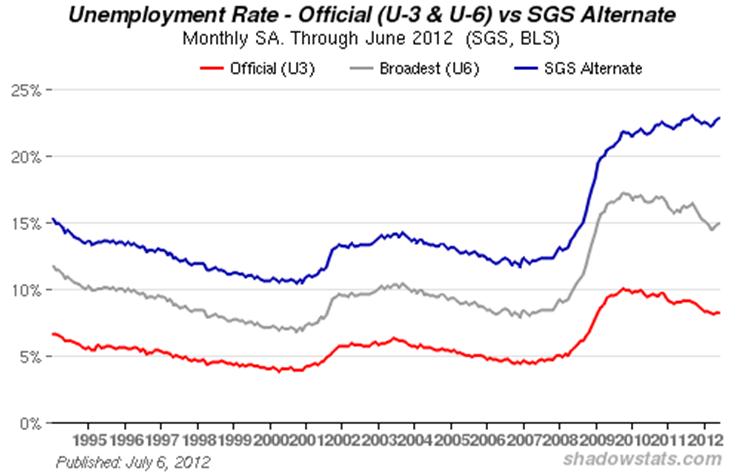
June Unemployment: 8.2% (U.3), 14.9% (U.6), 22.8% (Shadow Stats)
Shadow Stats Unemployment Nearing Cycle High
Year-to-Year M3 Money Supply Growth Notched Higher in June
__________
PLEASE NOTE: The next regular Commentary is scheduled for Friday, July 13th, covering the May trade deficit and June PPI.
Best wishes to all — John Williams
Opening Comments and Executive Summary. Even as published, the worse-than-expected softness in June’s payroll reporting is suggestive of weaker data ahead in key series, such as retail sales and industrial production, and possibly even in initial reporting of second-quarter 2012 GDP. There is a major distortion, though, in the reporting of both the payroll and household surveys: the use of concurrent seasonal factors by the Bureau of Labor Statistics (BLS), where the BLS does not publish consistent historical data that it otherwise calculates each and every month.
With nonfarm payrolls, the BLS does publish two months of revisions, along with enough detail for others to replicate the series calculations (see the Concurrent Seasonal Factor Distortions section in the Reporting Detail/Payroll Survey Detail). An analysis of the consistent but still unpublished data, however, shows an intensifying pattern of revised seasonal shifts of first-half data into second-half data. The June 2012 headline jobs growth of 80,000 was inflated simply by an unpublished shift of seasonal-factor effects into June from revised, but unreported, weakened seasonal-factor effects of earlier periods.
As to the headline unemployment rate, the BLS provides neither prior-period revisions nor underlying base data for independent calculations. As a result, the June headline unemployment rate of 8.2% was inconsistent with the May headline number of 8.2%. While the BLS internally has calculated the consistent number for May, it will not publish it. As a result, month-to-month comparisons—such as the current “unchanged”—are meaningless. Against consistent May reporting, the June headline unemployment rate might have risen; it might have fallen. Only the BLS knows what happened (see Commentary No. 451 and the Household Survey Detail section in Reporting Detail).
The seasonal-factor distortions affect only the adjusted, not the unadjusted data. Unfortunately, though, only the adjusted data can be used for the popularly-followed, month-to-month reporting.
Payroll Reporting. The headline 80,000 jobs gain for June was with minimal official revisions to April and May. May’s monthly gain was revised to 77,000 (previously 69,000), while April’s gain revised to 68,000 (previously 77,000). The plot of the nonfarm employment level continued to show no economic recovery to be in place.

Seasonally adjusted, the headline June U.3 unemployment rate of 8.2% officially was unchanged from May, while the broader U.6 rate widened to 14.9% from 14.8%, and the Shadow Stats alternate unemployment estimate widened to 22.8% in June, from 22.7% in May. The June Shadow Stats reading is closing in again on the cycle high of 23.0% seen in September 2011.
Hyperinflation Watch. Note: The general outlook is unchanged. Special Report No. 445 (June 12th) updated the hyperinflation outlook and the outlook for U.S. economic, U.S. dollar, and systemic-solvency conditions. The Special Report supplemented Hyperinflation 2012 (January 25th), which remains the primary missive detailing the hyperinflation story. This circumstance will be updated further as new developments unfold.
Money Supply M3 (June 2012). Based on over three weeks of reported data, the preliminary estimate of annual growth for the June 2012 SGS Ongoing-M3 Estimate—to be published tomorrow (July 7th) in the Alternate Data section—is on track to notch higher to 2.6% from 2.5% in May. With recent annual growth having peaked at 4.1% in January 2012, the upturn in annual broad money growth that began in February 2011 has faltered. Such a pattern—in an environment of massive Federal Reserve accommodation—continues to be suggestive of an intensifying systemic-solvency crisis.
The seasonally-adjusted, month-to-month change estimated for June M3 likely will be around 0.2%, versus 0.2% in May. The estimated month-to-month M3 changes, however, remain less reliable than the estimates of annual growth.
For June 2012, early estimates of year-to-year and month-to-month change follow for the narrower M1 and M2 measures (M2 includes M1, M3 includes M2). M2 for June is on track to show year-to-year growth of about 9.0%, versus a revised 9.5% in May, with month-to-month growth estimated at roughly 0.4%, the same as in May. The early estimate of M1 for June shows year-to-year growth of roughly 15.4%, versus a revised 15.9% (previously 16.0%) in May, with month-to-month change a likely gain of 0.3% in June, versus a 0.4% in May. The relatively stronger annual growth rates in M1 and M2 continue to reflect an earlier shifting of funds out of M3 accounts into M1 and M2 accounts.
__________
REPORTING DETAIL
EMPLOYMENT AND UNEMPLOYMENT (June 2012)
Payrolls Disappointed Market Expectations Still Again; “Unchanged” Headline Unemployment Rate Was Meaningless. Continuing downside surprises in payroll jobs growth appear to be reflecting a slowing base economy and increase the potential for downside reporting surprises in other major June economic reports, due for release in the next couple of weeks. Due to the inconsistent reporting of monthly unemployment rates (see Commentary No. 451), the official “unchanged” June unemployment rate was not necessarily so. Only the BLS knows what the actual change was, and they will not publish a hard number on that until December, when today’s number, itself, will have been revised (but not re-reported) six times, following whatever today’s consistent month-to-month change really was.
PAYROLL SURVEY DETAIL. The Bureau of Labor Statistics (BLS) reported today (July 6th) a statistically-insignificant, seasonally-adjusted June 2012 month-to-month payroll employment gain of 80,000 jobs (a gain of 79,000 before prior-period revisions) +/- 129,000 (95% confidence interval). The May payroll gain was revised to 77,000 (previously 69,000), while the April gain was revised to 68,000 (previously 77,000).
As discussed in Payroll Trends, the trend indication from the BLS seasonal-adjustment model suggests a 108,000 payroll gain for July, based on today’s reporting. While the trend indication often misses actual reporting (the indication for June was 113,000), it usually becomes the basis for the consensus outlook.
In terms of year-to-year change, the unadjusted June 2012 year-to-year growth in payrolls was 1.34%, versus an unrevised 1.39% in May, and a revised 1.30% (previously 1.29%) in April.

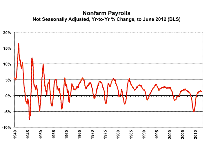
The preceding graphs of year-to-year unadjusted payroll change had shown a slowly rising trend in annual growth into 2011, which primarily reflected the still-protracted bottom-bouncing in the payroll series. That pattern of growth flattened out in late-2011, as shown in the first graph of the near-term detail in year-to-year change, and it has fluttered around a slightly lower level since April.
As shown in the longer-term graph (historical detail back to World War II), with the bottom-bouncing of recent years, current annual growth has recovered from the post-World War II record 5.06% decline in August 2009, which was the most severe annual contraction seen since the production shutdown at the end of World War II (a trough of a 7.59% annual contraction in September 1945). Disallowing the post-war shutdown as a normal business cycle, the August 2009 annual decline remains the worst since the Great Depression, yet the current level of employment is far from any recovery.
The regular graph of seasonally-adjusted payroll levels, which shows the current employment level well below its pre-2007 recession peak, is located in the Opening Comments and Executive Summary section.
Concurrent Seasonal Factor Distortions. Unreported, seasonally-adjusted monthly payroll numbers are showing a still-intensifying shift of first-half of the year jobs to the second-half of the year, as shown in the accompanying graph. The effect has been enough to help boost June’s employment reporting, based solely on shifting seasonal factors, as opposed to stronger economic activity.
Despite revisions in the monthly data each month that go back years, the BLS only publishes two months of revisions with each nonfarm payrolls release (April and May in the current instance), so as not to confuse data users. (The BLS publishes no revised data on a monthly basis for the household survey, despite similar seasonal-adjustment approach, as discussed in Commentary No. 451.) As a result, the reported April-through-June 2012 seasonally-adjusted payroll data are not consistent with earlier reporting. Conceivably, the shifting and unstable seasonal adjustments could move 80,000 jobs or more from earlier periods and insert them into the current period as new jobs, without there being any published evidence of that happening. The following graph suggests that something along those lines happened with June reporting.

The issues with the BLS’s concurrent seasonal factor adjustments and related inconsistencies in the monthly reporting of the historical time series are further discussed and detailed in the ShadowStats.com posting on May 2nd of Unpublished Payroll Data.
Incomplete and Inconsistent BLS Payroll Reporting. Five months have passed since the annual benchmark revisions to payroll employment, and the latest concurrent seasonal factors show renewed misreporting of the BLS’s own historical payroll levels, as well as ongoing instabilities in the BLS’s seasonal factors.
As discussed in prior writings (see Hyperinflation 2012, for example), seasonal-factor estimation for most economic series has been distorted severely by the extreme depth and duration of the economic contraction. These distortions are exacerbated for payroll employment data based on the BLS’s monthly seasonal-factor re-estimations and lack of full reporting.
Where the BLS recalculates the monthly seasonal factors each month for payroll employment, going back a number of years, outside of benchmarks, it only publishes the revised data for the last two months of reporting. The benchmark revision that accompanied the release of January 2012 payrolls, in theory, included a full update of the revised concurrent seasonally-adjusted data (actually it is off by a month or two). In the preceding graph, though, the latest revised (but not published by the BLS) adjusted payroll data show increasingly volatile, monthly seasonal-adjustment distortions of up to 80,000 jobs per month, with previously-reported payroll employment being shifted from the first-half to the second-half of the year, specifically with growth being shifted into June reporting. If seasonal-adjustment factors were stable in month-to-month reporting, which they should be under normal circumstances, then the graph of differences would be flat and at zero.
Note: A further big issue remains that the month-to-month seasonally-adjusted payroll data have become increasingly worthless, with reporting errors likely now well beyond the official 95% confidence interval of +/- 129,000 jobs in the reported monthly payroll change. Yet the media and the markets tout the data as meaningful, usually without question or qualification.
Birth-Death/Bias Factor Adjustment. Despite the ongoing and regular overstatement of monthly payroll employment—as evidenced usually by regular and massive, annual downward benchmark revisions (2011 excepted)—the BLS generally adds in upside monthly biases to the payroll employment numbers. The process was created simply by adding in a monthly “bias factor,” so as to prevent the otherwise potential political embarrassment of the BLS understating monthly jobs growth. The “bias factor” process resulted from an actual such embarrassment, with the underestimation of jobs growth coming out of the 1983 recession. That process eventually was recast as the now infamous Birth-Death Model (BDM), which purportedly models the effects of new business creation versus existing business bankruptcies.
June 2012 Bias. The not-seasonally-adjusted June 2012 bias was a positive 124,000, versus a positive 204,000 in May, and versus a current estimation of a 141,000 upside bias in June 2011. The aggregate upside bias for the last 12 months was 501,000, versus 518,000 in May and 525,000 in April. At present that is a monthly average of roughly 42,000 jobs created out of thin air, on top of some indeterminable amount of other jobs that are lost in the economy from business closings. Those losses simply are assumed away by the BLS as part of the BDM, as discussed below.
Problems with the Model. The aggregated upside annual reporting bias in the BDM reflects an ongoing assumption of a net positive jobs creation by new companies versus those going out business. Such becomes a self-fulfilling system, as the upside biases boost reporting for financial-market and political needs, with relatively good headline data, while often also setting up downside benchmark revisions for the next year, which traditionally are ignored by the media and the politicians. Where the BLS cannot measure the impact of jobs loss and jobs creation from employers starting up or going out of business, on a timely basis (within at least five years, if ever), such information is estimated by the addition of a bias-factor generated by the BDM.
Positive assumptions—commonly built into government statistical reporting and modeling—tend to result in overstated official estimates of general economic growth. Along with happy guesstimates, there usually are underlying assumptions of perpetual economic growth in most models. Accordingly, the functioning and relevance of those models become impaired during periods of economic downturn, and the current downturn has been the most severe—in depth as well as duration—since the Great Depression.
Indeed, historically, the BDM biases have tended to overstate payroll employment levels—to understate employment declines—during recessions. There is a faulty underlying premise here that jobs created by start-up companies in this downturn have more than offset jobs lost by companies going out of business. So, if a company fails to report its payrolls because it has gone out of business, the BLS assumes the firm still has its previously-reported employees and adjusts those numbers for the trend in the company’s industry.
Further, the presumed net additional “surplus” jobs created by start-up firms, get added on to the payroll estimates each month as a special add-factor. These add-factors are set now to add an average of about 42,000 jobs per month in the current year, but the actual overstatement of monthly jobs likely exceeds that number by a significant amount. With the underlying economy continuing to falter, I expect a significant downside benchmark revision for 2012 (based on the upcoming March 2012 benchmark that will be published in 2013), given current details of the BLS’s overly positive estimates.
HOUSEHOLD SURVEY DETAILS. As discussed in Commentary No. 451, seasonally-adjusted month-to-month comparisons of components in the household survey having no meaning. The “unchanged” nature of the June unemployment rate could have been that, but the headline number just as easily could have shown an increase or a decrease. There is no way to tell, given current BLS reporting policies; the BLS calculates but does not report consistent data as part of the monthly estimation process.
The headline numbers published here each month simply are not consistent and not comparable with the numbers published the month before, except in December, when the monthly data are restated for seasonal-factor revisions. At present—partially as a result of the severity of the economic downturn—seasonal factors are highly volatile and unstable. The BLS uses “concurrent” seasonal factor adjustments in the household survey, but, with that process, all adjusted monthly data are recalculated going back a number of years, each and every month.
As discussed in the Concurrent Seasonal Factor Distortions section above, on the payroll survey, at least the BLS publishes two months of revisions along with the headline payroll number. The BLS also makes available enough detail so that private analysts can calculate the entire revised series. That is not the case with the household series, where the monthly headline numbers are standalone and fully inconsistent with the prior month’s estimations. All this said, following are the meaningless seasonally-adjusted numbers that will cause today’s markets to gyrate, will excite the popular press and will lead political candidates to pontificate. Separately, the unadjusted numbers are consistent in their preparation.
Headline Household Employment. Based on the June household survey, which counts the number of people with jobs, as opposed to the payroll survey that counts the number of jobs (including multiple job holders more than once) June 2012 employment rose by 128,000, versus the May estimate of 422,000. As discussed above, the headline, seasonally-adjusted monthly change here is meaningless, due to the underlying data being inconsistent on a month-to-month basis.
Unemployment Rates. The reported June 2012 seasonally-adjusted headline (U.3) unemployment rate of 8.22% virtually was unchanged from the 8.21% that was separately and inconsistently estimated for May. The official 95% confidence interval for the headline number is +/- 0.23% percentage point. As discussed above, however, the headline monthly change here is worthless, due to underlying data inconsistencies. On an unadjusted basis, June’s U.3 unemployment rate was 8.4%, versus May’s 7.9%.
The broadest unemployment rate published by the BLS, U.6 includes accounting for those marginally attached to the labor force (including short-term discouraged workers) and those who are employed part-time for economic reasons (they cannot find a full-time job).
The June U.6 unemployment rate rose to a seasonally-adjusted 14.9%, versus 14.8% in May. The unadjusted June U.6 rate rose to 15.1%, up from 14.3% in May.
Discouraged Workers. The count of short-term discouraged workers (never seasonally-adjusted) declined slightly in June to 821,000, from 830,000 in May. That reflected the balance of the headline unemployed—increasingly giving up looking for work—leaving the U.3 unemployment category and being rolled into the U.6 measure as short-term “discouraged workers,” versus those moving from short-term status into the netherworld of long-term discouraged-worker status. It is the long-term discouraged worker category that defines the SGS-Alternate Unemployment Measure.
In 1994, during the Clinton Administration, “discouraged workers”—those who had given up looking for a job because there were no jobs to be had—were redefined so as to be counted only if they had been “discouraged” for less than a year. This time qualification defined away the long-term discouraged workers. The remaining short-term discouraged workers (less than one year) are included in U.6.
Adding the SGS estimate of excluded long-term discouraged workers back into the total unemployed and labor force, unemployment—more in line with common experience as estimated by the SGS-Alternate Unemployment Measure—rose to 22.8% in June, which is closing in on the current cycle high of 23.0% seen in September 2011. The Mat estimate was 22.7%. The SGS estimate generally is built on top of the official U.6 reporting, and tends to follow its relative monthly movements. Accordingly, the SGS measure will suffer some of the current seasonal-adjustment woes afflicting the base series.
There continues to be a noticeable divergence in the Shadow Stats series versus U.6. The reason for this is that U.6, again, only includes discouraged workers who have been discouraged for less than a year. As the discouraged-worker status ages, those that go beyond one year fall off the government counting, and new workers enter “discouraged” status. Accordingly, with the continual rollover, the flow of headline workers continues into the short-term discouraged workers (U.6), and from U.6 into long-term discouraged worker status (Shadow Stats Measure), at what has been an accelerating pace. See the Alternate Data tab for more detail.
As discussed in previous writings, an unemployment rate above 22% might raise questions in terms of a comparison with the purported peak unemployment in the Great Depression (1933) of 25%. The SGS level likely is about as bad as the peak unemployment seen in the 1973 to 1975 recession. The Great Depression unemployment rate was estimated well after the fact, with 27% of those employed working on farms. Today, less that 2% work on farms. Accordingly, for purposes of Great Depression comparison, I would look at the estimated peak nonfarm unemployment rate in 1933 of 34% to 35%.
Week Ahead. Market recognition of an intensifying double-dip recession has started to take a stronger hold, at the moment, while recognition of a mounting inflation threat remains sparse. The political system would like to see the issues disappear until after the election; the media does its best to avoid publicizing unhappy economic news or to put a happy spin on the numbers; and the financial markets will do their best to avoid recognition of the problems for as long as possible, problems that have horrendous implications for the markets and for systemic stability.
Until such time as financial-market expectations move to catch up fully with underlying reality, or underlying reality catches up with the markets, reporting generally will continue to show higher-than-expected inflation and weaker-than-expected economic results in the months and year ahead. Increasingly, previously unreported economic weakness should show up in prior-period revisions.
U.S. Trade Balance (May 2012). Details of the May trade deficit will be released on Wednesday, July 11th. In combination, the April and May data will serve as the proxy for the full second-quarter trade deficit and the basis for the net-export-account estimate in the initial reporting of second-quarter 2012 GDP on July 27th.
The May deficit likely will be wider than market expectations, with implications for a negative impact on the advance GDP headline number.
Producer Price Index—PPI (June 2012). The June PPI is scheduled for release on Friday, July 13th. Although seasonal adjustments tend to add some upside to energy prices at this time of year, oil prices and related gasoline prices tumbled enough in June, on an unadjusted basis, to generate a monthly contraction in the headline PPI, which otherwise shows somewhat random volatility.
__________