COMMENTARY NUMBER 534
May CPI, Housing Starts, Real Retail Sales, Real Earnings, Systemic Solvency

June 18, 2013

__________

Fed’s Expanded QE3 Has Monetized 78.4% of the Concurrent Increase in Treasury Debt

Relationship of Post-2008 Monetary Base Activity to Broad Money Supply

May Year-to-Year Inflation: 1.4% (CPI-U), 1.2% (CPI-W), 9.0% (ShadowStats)

Real Retail Sales Still Signal Broad Economic Downturn

Second-Quarter Housing Starts on Track for Quarterly Plunge

__________

 

PLEASE NOTE: The next regular Commentary is scheduled for Tuesday, June 25th, covering May new orders for durable goods and new- and existing-home sales.

Best wishes to all — John Williams

 

OPENING COMMENTS AND EXECUTIVE SUMMARY

Amid rumors that the Federal Open Market Committee (FOMC) is close to indicating some pullback in the Fed’s quantitative easing program QE3—perhaps announcing same following tomorrow’s (June 19th) FOMC meeting—the U.S. economy is showing early signs of a second-quarter 2013 contraction; headline consumer inflation remains contained; and ongoing banking-system stress is suggested in the latest monetary data.  Accordingly, unless the forthcoming FOMC announcement includes a specific shift to less-accommodative policy actions, any carefully worded changes in the FOMC statement—suggestive of a shift in policy—could be viewed as of limited substance, no more than continuing jawboning.  The Fed remains locked into quantitative easing by stresses in the banking system, and by the continuing political cover provided by a weakening economy.

The expansion of QE3, at the beginning of calendar-year 2013, encompassed new purchasing of U.S. Treasury securities.  To date (June 12th), the Federal Reserve effectively has monetized 78.4% of net new U.S. Treasury debt since January 2, 2013.  With the U.S. Treasury playing accounting games that should hold the gross federal debt at its debt ceiling through Labor Day, the Fed’s monetization should top 100% of net issuance, year-to-date, within the next two months.  Even so, at the onset of the current debt-ceiling limitations on new issuance, the Fed’s monetization year-to-date (May 20th) already was at 69.3%.

Banking System Under Stress?  Year-to-year change in money supply versus monetary base is detailed in the Hyperinflation Watch section.  In the post-2008 period of extreme accommodation by the Fed, there has been some correlation between annual growth in the St. Louis Fed’s monetary base and annual in M3, as measured by the ShadowStats-Ongoing M3 Estimate.  The correlations between the growth rates are 58.1% for M3, 39.9% for M2 and 36.7% for M1, on a coincident basis.

 

While there has been no significant flow-through to the broad money supply from the expanded monetary base—banks still are not lending normally into the regular flow of commerce—there appears to have been some minor effect.  The ShadowStats contention has been that the Fed’s easing activity has been aimed primarily at supporting banking-system solvency and liquidity, not at propping the economy or containing inflation.  When the Fed boosts its easing, but money growth slows, as seen at present, there is a potential indication there of mounting financial stress within the banking system.  More will follow on this in later missives.

 

May 2013 Inflation and Economic Activity: Bottoming Inflation, Contracting Economy.  On the inflation front, both the headline PPI and the CPI turned to the plus side in May, as the distorting seasonal factors—tied to energy inflation—began to migrate from inflation-suppression to inflation-boosting.  The impact on headline inflation reporting should be heavily to the upside for the next several months.  Separately, as recent dollar strength has started to wane, oil prices again are pushing higher—tied both to currencies and to Middle Eastern tensions.  Inflationary pressures should continue to mount from U.S. dollar problems (see Hyperinflation Summary), not from an economic recovery.

Indeed, the economy is slowing.  Although May payrolls were near-consensus, and retail sales topped consensus, they still were weak.  May industrial production (see Commentary No. 533) and housing starts both suggested that a second-quarter contraction was beginning to unfold.  Consumer liquidity remains severely impaired, and the impact of that will be in an intensifying economic downturn, not in a near-term economic recovery

Consumer Price Index—May 2013.  Reflecting the beginning of the annual shift in seasonal adjustments, from suppressing to boosting energy-related inflation, headline consumer inflation in May notched higher on a monthly basis and jumped in annual terms.  In June reporting, those still-shifting energy-related seasonals will provide a significant boost to headline inflation. 

Despite these increasingly unstable seasonal adjustments, which heavily distort the monthly headline inflation numbers, year-to-year inflation numbers are not seasonally adjusted.  That said, however, there are other issues in terms of methodological changes—made to the series in recent decades—that were designed to understate the government’s reporting of consumer inflation, as discussed in the Public Comment on Inflation Measurement.

CPI-U.  The headline, seasonally-adjusted CPI-U for May 2013 rose by 0.15%, which was shy by 0.00053% of rounding up to a headline 0.2% increase, instead of down to 0.1%.  Unadjusted monthly May inflation was 0.18% (still affected by less-severe, negative energy seasonals).  In April, the CPI-U fell by 0.37% for the month (down by 0.10% unadjusted).  Not seasonally adjusted, May 2013 year-to-year inflation for the CPI-U was 1.36%, up from 1.06% in April.

Core CPI-U.  Seasonally-adjusted May 2013 “core” CPI-U inflation (net of food and energy inflation) rose by 0.17% (0.10% unadjusted) month-to-month, versus an adjusted 0.05% (0.08% unadjusted) gain in April.  The unadjusted, year-to-year core rate eased to 1.68% in May from 1.72% in April.  The CPI core annual inflation number generally was in line with the core-PPI growth, which was 1.65% in May, following 1.71% annual inflation in April (see Reporting Detail for graph).

CPI-W.  The May 2013 headline, seasonally-adjusted CPI-W, which is a narrower series and has greater weighting for gasoline than does the CPI-U, rose by 0.16% (up by 0.20% unadjusted), for the month, versus an adjusted decline of 0.49% (down by 0.16% unadjusted) in April.  Unadjusted, May 2013 year-to-year CPI-W inflation was 1.24%, up from an annual 0.85% increase in April.

Chained-CPI-U.  The initial reporting of unadjusted, year-to-year inflation for the May 2013 C-CPI-U was 1.31%, up from 1.09% in April.

Alternate Consumer Inflation Measures.  Adjusted to pre-Clinton methodologies—the ShadowStats-Alternate Consumer Inflation Measure (1990-based)—annual CPI inflation was roughly 4.8% in May 2013, up from 4.5% in April 2013.  The ShadowStats-Alternate Consumer Inflation Measure (1980-Based), which reverses gimmicked changes to official CPI reporting methodologies back to 1980, rose to about 9.0% in May 2013, versus an annual inflation rate of 8.7% in April 2013.

Real (Inflation-Adjusted) Retail Sales—May 2013.  With a 0.15% monthly gain the May CPI-U, the nominal (not-adjusted-for-inflation) headline gain of 0.55% in May retail sales was a 0.40% gain, in real terms, after adjustment for inflation.  The revised headline monthly nominal sales gain of 0.15% for April reflected a real gain of 0.52%, given the monthly decline of 0.37% in the April CPI-U.  See Commentary No. 532 for nominal reporting detail on May retail sales.

Year-to-year, May 2013 real retail sales rose at an annual pace of 2.88%, versus an unrevised annual gain of 2.52% in April.  In normal economic times, recent levels of annual real growth would be signaling a pending recession.  In the current circumstance, this signal likely will serve as an indicator of a renewed downturn in broad economic activity.

As official consumer inflation resumes its seasonally-adjusted upturn, and as overall retail sales continue to suffer from an intensifying consumer-liquidity squeeze, these data should trend meaningfully lower, in what eventually will gain recognition as a formal, double-dip recession.

As discussed below and in Commentary No. 532, there has been no change in the underlying consumer-liquidity structural problems that are constraining consumption.  There is nothing that would support a sustainable turnaround in retail sales, personal consumption, housing or general economic activity.  There never was a broad economic recovery, and there is no recovery underway, just general bottom-bouncing that is turning down anew.

The first graph following reflects official real retail sales reporting, which, at least temporarily, has topped its pre-recession level.  That pattern does not hold, however, if the series is corrected for understated inflation, as shown in the second graph.  Corrected for the use of understated inflation rates used in the economic deflation process, a renewed downturn in activity—following an extended period of low-level stagnation—actually began in second- or third-quarter 2012.

Corrected Retail Sales.  The first graph reflects real retail sales as usually reported by the St. Louis Fed, deflated by the CPI-U, but it is indexed to January 2000 = 100.  ShadowStats did the deflation using the May 2013 CPI-U release.  The CPI-U, however, understates inflation (see the Public Comment on Inflation), with the effect of overstating inflation-adjusted growth.  Instead of being deflated by the CPI-U, the “corrected” real retail numbers in the second graph use the ShadowStats-Alternate Inflation Measure (1990-Base) for deflation.

As discussed in Hyperinflation 2012 and Special Commentary (No. 485), with the higher inflation of the ShadowStats measure, the revamped numbers show a pattern of plunge and stagnation, consistent with patterns seen in real median household income and consumer confidence measures.  The recent topping-out reverted to renewed decline in second-quarter 2012, in this series that had been bottom-bouncing along a low-level plateau of economic activity since the economic collapse from 2006 into 2009.

Consumer Liquidity Issues Updated.  Further to the comments and graphs in Commentary No. 532 on structural impairments to consumer liquidity, the following two graphs update the latest consumer information.  A consumer without income growth, without the ability to expand credit, and without the willingness to spend money, cannot fuel economic recovery in retail sales, housing or GDP.

Real (Inflation-Adjusted) Average Weekly Earnings—May 2013.  Deflated by the CPI-W, real (inflation-adjusted) average weekly earnings for production and nonsupervisory employees series, in May 2013, rose by 0.2% for the month, following a 0.3% monthly gain in April.  The April gain was due to negative monthly inflation, the May gain was due to an increase in average working hours.

Unadjusted and year-to-year, May 2013 real earnings gained 0.6%, versus an annual 0.3% decline in April.  Both the monthly and annual fluctuations in this series are irregular, and current reporting remains well within the normal bounds of volatility.

The preceding graph of real average weekly earnings shows the earnings as officially deflated by the BLS (red-line), and as adjusted for the ShadowStats-Alternate CPI Measure, 1990-based (blue-line).  When inflation-depressing methodologies of the 1990s began to kick-in, the artificially weakened CPI-W (also used in calculating Social Security cost-of-living adjustments) helped to prop up the reported real earnings. 

Official real earnings today still have not recovered their inflation-adjusted levels of the early-1970s, and, at best, have been flat for the last decade.  Deflated by the ShadowStats measure, real earnings have been in fairly regular decline for the last four decades, which is much closer to common experience than the pattern suggested by the CPI-W.  See Public Commentary on Inflation Measurement for further detail.

Consumer Sentiment—Preliminary June 2013.  The early estimate for June consumer sentiment, as published by the University of Michigan, reportedly eased back minimally from the full-month’s estimate for May.  With the extreme monthly volatility in the series smoothed, sentiment has not joined in the GDP’s purported recovery.  Instead, the levels here, as well as in consumer confidence (see Commentary No. 532), remain near the lows seen in historic recessions.

Residential Investment/Housing Starts—May 2013.  With no meaningful recovery from April’s statistically-significant plunge in monthly activity, May housing starts reporting suggested that second-quarter 2013 is on track to show a quarterly plunge in housing activity.  The 6.8% headline gain in May 2013 housing starts was statistically-insignificant, as were the headline 0.3% gain in one-unit housing starts, and the headline 24.9% gain in the five-units-or-more category.  Those gains followed revised respective monthly contractions of 14.7% (total), 4.2% (one-unit) and 31.2% (five-units-or-more).

In combination, though, the two months of second-quarter data have set an ominous monthly pattern for housing starts, suggestive of an outright quarterly plunge.  April and May starts have averaged 885.0 thousand so far in second-quarter 2013.  That is against an average of 957.3 thousand in first-quarter 2013 and 896.3 thousand in fourth-quarter 2012.  If the second-quarter numbers held at their current average, that would represent an annualized quarterly decline of 27.0% (same way the GDP growth is calculated) in aggregate housing starts.

The official reporting of housing starts is expressed at an annualized monthly pace of starts, which was 914,000 in May 2013, following an 856,000 pace in April.  Graphs on that basis are plotted in the Reporting Detail section.  Due to the regular, extreme volatility in this monthly series, however, it is more meaningful to look at the actual, non-annualized monthly number.  The graphed and quarterly patterns are the same; it is just that the monthly levels tend to be a little more realistic.  Accordingly, the following graphs reflect the seasonally-adjusted monthly rates, not the annualized numbers.

As shown in the following graph, although May aggregate activity remained well above the record monthly low seen for the present series in April 2009, the May 2013 headline number still was 60% below the January 2006 series high.

This highly-volatile and irregular housing starts series tends to show mixed patterns, partially because it is reported as a mix of residential construction products, with one-unit housing starts that generally are for individual consumption resulting in new home sales, versus multi-unit starts that generally reflect the building of rental and apartment units.  The aggregate May gain of 6.8% was composed of a statistically-insignificant 0.3% gain in one-unit housing starts, combined with a statistically-insignificant 21.6% monthly gain in starts of multiple-unit structures.  The preceding graph reflects that detail

The next two graphs break-up the component reporting between one-unit and multiple-unit housing starts.  The Census Bureau breaks its headline data into three categories beyond “total.”  Those structure definitions are “1 unit,” “2 to 4 units,” and “5 units or more.”  Due to lack of “meeting reliability standards,” Census does not publish the actual numbers for the “2 to 4 units,” although the numbers could be imputed.  Accordingly, ShadowStats breaks the data into two sub-categories: “single-unit” and “multiple-unit” starts, where the multiple-unit category simply is the total unit count, minus the single-unit count.

Activity in single-unit starts generally has remained stagnant in the post-housing-crash environment, and has headed lower, recently.  Multiple-unit starts activity has remained highly unstable and irregular, though trending higher.  With the private-housing market difficulties, former homeowners or those not entering the home-owning market have pushed up demand for rental units.  In the context of extreme volatility, multiple-unit starts have moved irregularly to pre-crash levels in recent reporting.

 

[For further detail on the May CPI and related series, and May housing starts,
 see the Reporting Detail section.]

 

 

__________

 

 

 

HYPERINFLATION WATCH

 

Monetization and Monetary Base.  Along with the Federal Reserve having monetized 78.4% of the issuance of gross federal debt by the U.S. Treasury year-to-date (calendar year 2013), the monetary base has continued to soar, both in terms of level and year-to-year growth, as reflected in the accompanying graphs.  At the same time, annual growth has started to slow for the broad money supply (M3), as provided in the ShadowStats Ongoing-M3 Estimate, for May 2013.  Discussed and graphed in the Opening Comments section, there is a relationship between growth in the monetary base and the growth in M3.  When the patterns begin to show sharp divergence, such can signal mounting liquidity stresses in the banking system.

Based on full reporting for May 2013, annual M3 growth slowed to 4.2% in May, versus 4.4% in April.  While the slowing is not large, it is in the opposite direction of what might be expected from QE3 and with the Fed’s increasing monetization of U.S. Treasury debt.  The variance between the behavior of M3 and the monetary base is a result of the lack of normal bank lending, and the nature of the increasing variance is suggestive of mounting banking-system instabilities.  It is in the promotion of banking-system stability, not in attempting to lower unemployment or to contain inflation, that Mr. Bernanke introduced his quantitative easing (see No. 527: Special Commentary).  Accordingly, there is nothing here to suggest an imminent end to QE3.

 

 

 

 

 

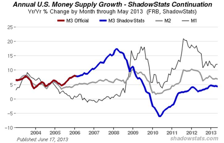
The monetary base has been setting successive historic highs, both in terms of level, and in terms of year-to-year growth in the new cycle.  As shown in the accompanying graphs, the monetary base was at a seasonally-adjusted (SA) two-week average level of $3,245.2 billion as of June 12th, a record-high.  The 21.2% pace of rising year-to-year growth has not been seen in two years, when QE2 was exploding. 

The monetary base is currency in circulation (part of M1 money supply) plus bank reserves (not part of the money supply) (see a more-complete definition in the Money Supply Special Report).  Traditionally, the Federal Reserve has used the monetary base to increase or decrease growth in the money supply, but such has not had its normal impact in the post-2008 crisis period.  Instead, financially troubled banks have been holding their excess reserves with the Federal Reserve, not lending the available cash into the normal flow of commerce.  When the Fed monetizes U.S. Treasury securities, as it has been doing, that usually adds directly to the broad money supply, and it contributes to selling pressure against the U.S. dollar.  Faltering year-to-year broad money supply growth in this circumstance, as seen at present, tends to be an indication of mounting systemic stress in the banking industry.

 

Hyperinflation Outlook—Unchanged Summary.  The hyperinflation outlook was revised and updated with new detail on May 29th, in No. 527: Special Commentary, and this summary was revised and expanded to reflect the content of that Special Commentary in Commentary No. 531 of June 8th.  The following text has not been changed since No. 531.  It is intended as background material for new subscribers and for those looking for a brief summary of the broad outlook of the economic, systemic and inflation crises that face the United States in the year or so ahead.

Background Material.  No. 527: Special Commentary (May 2013) supplemented No. 485: Special Commentary (November 2012), reviewing shifting market sentiment on a variety of issues affecting the U.S. dollar and prices of precious metals.  No. 485, in turn, updated Hyperinflation 2012 (January 2012)—the base document for the hyperinflation story—and the broad outlook for the economy and inflation, as well as for systemic-stability and the U.S. dollar.  Of some use, here, also is the Public Comment on Inflation.

These are the primary articles outlining current conditions and the background to the hyperinflation forecast, and they are suggested reading for subscribers who have not seen them and/or for those who otherwise are trying to understand the basics of the hyperinflation outlook.  The fundamentals have not changed in recent years, other than events keep moving towards the circumstance of a domestic U.S. hyperinflation by the end of 2014.  Nonetheless, the next, fully-updated hyperinflation report is targeted for publication late this month (June 2013). 

Beginning to Approach the End Game.  Nothing is normal: not the economy, not the financial system, not the financial markets and not the political system.  The financial system still remains in the throes and aftershocks of the 2008 panic and near-systemic collapse, and from the ongoing responses to same by the Federal Reserve and federal government.  Further panic is possible and hyperinflation remains inevitable. 

Typical of an approaching, major turning point in the domestic- and global-market perceptions, bouts of extreme volatility and instability have been seen with increasing frequency in the financial markets, including equities, currencies and the monetary precious metals (gold and silver).  Consensus market expectations on the economy and Federal Reserve policy also have been in increasing flux, but the markets are stuck with underlying reality and, eventually, they will have to recognize same.  The economy remains in continued and deepening trouble, and the Federal Reserve—despite currency-market platitudes to the contrary—is locked into quantitative easing by persistent problems now well beyond its control. 

At the same time, rapidly deteriorating expectations for domestic political stability reflect widening government scandals, in addition to the dominant global-financial-market concern of there being no viable prospect of those controlling the U.S. government addressing the long-range sovereign-solvency issues of the United States government.  All these factors, in combination, show the end game to be nearing. 

The most visible and vulnerable financial element to suffer early in this crisis likely will be the U.S. dollar in the currency markets (all dollar references here are to the U.S. dollar, unless otherwise stated).  Heavy dollar selling should evolve into massive dumping of the dollar and dollar-denominated paper assets.  Dollar-based commodity prices, such as oil, should soar, accelerating the pace of domestic inflation.  In turn, that circumstance likely will trigger some removal of the U.S. dollar from its present global-reserve-currency status, which would further exacerbate the currency and inflation problems tied to the dollar.

This still-forming great financial tempest has cleared the horizon; its impact on the United States and those living in a dollar-based world will dominate and overtake the continuing economic and systemic-solvency crises of the last eight years.  The issues that never were resolved in the 2008 panic and its aftermath are about to be exacerbated.  Based on the precedents established in 2008, likely reactions from the government and the Fed would be to throw increasingly worthless money at the intensifying crises.  Attempts to save the system all have inflationary implications.  A domestic hyperinflationary environment should evolve from something akin to these crises before the end of next year (2014).  The shifting underlying fundamentals are discussed in No. 527: Special Commentary; some of potential breaking crises will be expanded upon in the next revision to the hyperinflation report.

Still Living with the 2008 Crisis.  There never was an actual recovery following the economic downturn that began in 2006 and collapsed into 2008 and 2009.  What followed was a protracted period of business stagnation that began to turn down anew in second- and third-quarter 2012 (see new detail in Commentary No. 530).  The official recovery seen in GDP has been a statistical illusion generated by the use of understated inflation in calculating key economic series (see No. 527: Special Commentary, Commentary No. 528 and Public Comment on Inflation).  Nonetheless, given the nature of official reporting, the renewed downturn likely will gain recognition as the second-dip in a double- or multiple-dip recession.

What continues to unfold in the systemic and economic crises is just an ongoing part of the 2008 turmoil.  All the extraordinary actions and interventions bought a little time, but they did not resolve the various crises.  That the crises continue can be seen in deteriorating economic activity and in the ongoing panicked actions by the Federal Reserve, where it still proactively is monetizing U.S. Treasury debt at a pace suggestive of a Treasury that is unable to borrow otherwise. 

Before and since the mid-April rout in gold prices, there had and has been mounting hype about the Fed potentially pulling back on its “easing” and a coincident Wall Street push to talk-down gold prices.  As discussed in No. 527: Special Commentary, those factors appear to be little more than platitudes to the Fed’s critics and intensified jawboning to support the U.S. dollar and to soften gold, in advance of the still-festering crises in the federal-budget and debt-ceiling negotiations.  Despite orchestrated public calls for “prudence” by the Fed, the underlying and deteriorating financial-system and economic instabilities have self-trapped the Fed into an expanding-liquidity or easing role that likely will not be escaped until the ultimate demise of the U.S. dollar. 

Further complicating the circumstance for the U.S. currency is the increasing tendency of major U.S. trading partners to move away from using the dollar in international trade, such as seen most recently in the developing relationship between France and China (see No. 527: Special Commentary).

The Fed’s recent and ongoing liquidity actions themselves suggest a signal of deepening problems in the financial system.  Mr. Bernanke admits that the Fed can do little to stimulate the economy, but it can create systemic liquidity and inflation.  Accordingly, the Fed’s continuing easing moves appear to have been primarily an effort to prop-up the banking system and also to provide back-up liquidity to the U.S. Treasury, under the political cover of a “weakening economy.”  Mounting signs of intensifying domestic banking-system stress are seen in softening annual growth in the broad money supply, despite a soaring pace of annual growth in the monetary base, and in global banking-system stress that followed the crisis in Cyprus and continuing, related aftershocks.

Still Living with the U.S. Government’s Fiscal Crisis.  Again, as covered in No. 527: Special Commentary, the U.S. Treasury is in the process of going through extraordinary accounting gimmicks, at present, in order to avoid exceeding the federal-debt ceiling.  Early-September appears to be the deadline for resolving the issues tied to the debt ceiling, including—in theory—significant budget-deficit cuts.

Both Houses of Congress recently put forth outlines of ten-year budget proposals that still are shy on detail.  The ten-year plan by the Republican-controlled House proposes to balance the cash-based deficit as well as to address issues related to unfunded liabilities.  The plan put forth by the Democrat-controlled Senate does not look to balance the cash-based deficit.  Given continued political contentiousness and the use of unrealistically positive economic assumptions to help the budget projections along, little but gimmicked numbers and further smoke-and-mirrors are likely to come out of upcoming negotiations.  There still appears to be no chance of a forthcoming, substantive agreement on balancing the federal deficit.

Indeed, ongoing and deepening economic woes assure that the usual budget forecasts—based on overly-optimistic economic projections—will fall far short of fiscal balance and propriety.  Chances also remain nil for the government fully addressing the GAAP-based deficit that hit $6.6 trillion in 2012, let alone balancing the popularly-followed, official cash-based accounting deficit that was $1.1 trillion in 2012 (see No. 500: Special Commentary).

Efforts at delaying meaningful fiscal action, including briefly postponing conflict over the Treasury’s debt ceiling, bought the politicians in Washington minimal time in the global financial markets, but the time has run out and patience in the global markets is near exhaustion.  The continuing unwillingness and political inability of the current government to address seriously the longer-range U.S. sovereign-solvency issues, only pushes along the regular unfolding of events that eventually will trigger a domestic hyperinflation, as discussed in Commentary No. 491. 

U.S. Dollar Remains Proximal Hyperinflation Trigger.  The unfolding fiscal catastrophe, in combination with the Fed’s direct monetization of Treasury debt, eventually (more likely sooner rather than later) will savage the U.S. dollar’s exchange rate, boosting oil and gasoline prices, and boosting money supply growth and domestic U.S. inflation.  Relative market tranquility has given way to mounting instabilities, and severe market turmoil likely looms, despite the tactics of delay by the politicians and ongoing obfuscation by the Federal Reserve. 

This should become increasingly evident as the disgruntled global markets begin to move sustainably against the U.S. dollar.  As discussed earlier, a dollar-selling panic is likely this year—still of reasonably high risk in the next month or so—with its effects and aftershocks setting hyperinflation into action in 2014.  Gold remains the primary and long-range hedge against the upcoming debasement of the U.S. dollar, irrespective of any near-term price gyrations in the gold market.

The rise in the price of gold in recent years was fundamental.  The recent panicked sell-off in gold was not.  With the underlying fundamentals of ongoing dollar-debasement in place, the upside potential for gold, in dollar terms, is limited only by its inverse relationship to the purchasing power of the U.S. dollar (eventually headed effectively to zero).  Again, physical gold—held for the longer term—remains as a store of wealth, the primary hedge against the loss of U.S. dollar purchasing power. 

 

Monthly Gold Graphs.  Following are the regular graphs of gold prices versus the Swiss franc, oil prices and silver prices that usually accompany the Commentary on the monthly CPI release.  The recent rally in the U.S. dollar largely has faded, and oil prices have started to move higher in response to renewed dollar weakness and to increasing political instabilities in the Middle East.  Gold and silver prices remain weak, but the underlying fundamentals there could not be stronger.  The “latest June” points in the following graphs are mid-day (New York) market prices, or London afternoon or daily fixes for gold and silver, as of June 18th.

 

 

 

__________

 

 

 

REPORTING DETAIL

 

 

CONSUMER PRICE INDEX—CPI (May 2013)

Consumer Inflation Resurfaced in May, Minimally, With More-Friendly Energy-Price Seasonal Factors.  Reflecting the beginning of a shift in seasonal adjustments from suppressing to boosting adjusted energy-related inflation, headline consumer inflation notched higher on a monthly basis and jumped in annual terms.  Next month, the energy-related seasonals will provide a significant boost to the headline inflation. 

Where these increasingly unstable seasonal adjustments have become, and will remain, heavily distorting of the headline inflation numbers, the year-to-year inflation numbers are not seasonally adjusted.  That said, there are other issues in terms of methodological changes—made to the series in recent decades—that were designed to understate the government’s reporting of consumer inflation, as discussed in the Public Comment on Inflation Measurement.

 

CPI-U.  The Bureau of Labor Statistics (BLS) reported on June 18th that the seasonally-adjusted CPI-U for May 2013 rose by 0.15%, which was shy by 0.00053% of rounding up to a headline 0.2% increase, instead of down to 0.1%.  Unadjusted, month-to-month May inflation was 0.18%.  In April, the CPI-U fell by 0.37% for the month (down by 0.10% unadjusted).  As happens at this time of year, seasonal adjustments again suppressed energy-related inflation, but the trend has started to shift, and those seasonal-factor reporting distortions flip to the upside with next month’s reporting.

Per the BLS, a 0.8% monthly increase (1.0% increase per the more-comprehensive Department of Energy surveying) in not-seasonally-adjusted gasoline prices for May 2013 was turned to unchanged, by irregular and seasonal-adjustment factors.

In terms of the headline CPI-U monthly gain of 0.1% (0.2% unadjusted), the aggregate energy inflation in May 2013 showed an adjusted 0.4% (unadjusted 1.2%) monthly gain.  In the other major CPI sectors, there was a not-credible 0.1% monthly decline in food inflation, both before and after seasonal adjustments, and an adjusted 0.2% (unadjusted 0.1%) monthly increase in “core” inflation.

Not seasonally adjusted, May 2013 year-to-year inflation for the CPI-U was 1.36%, up from 1.06% in April.

Year-to-year, CPI-U inflation would increase or decrease in next month’s June 2013 reporting, dependent on the seasonally-adjusted monthly change, versus a reported 0.12% gain in monthly inflation for June 2012.  The adjusted change is used here, since that is how consensus expectations are expressed.  To approximate the annual unadjusted inflation rate for June 2013, the difference in June’s headline monthly change (or forecast of same), versus the year-ago monthly change, should be added to or subtracted directly from the May 2013 annual inflation rate of 1.36%.

Core CPI-U.  Seasonally-adjusted May 2013 “core” CPI-U inflation (net of food and energy inflation) rose by 0.17% (0.10% unadjusted) month-to-month, versus an adjusted 0.05% (0.08% unadjusted) gain in April.

Twenty-one of the last thirty months have shown rising year-to-year, or annual, core CPI-U inflation, with the year-to-year core rate easing to 1.68% in May from 1.72% in April.  The CPI core annual inflation number generally was in line with the core-PPI growth, which was 1.65% in May, following 1.71% annual inflation in April.

The May 2013 CPI-U year-to-year core rate still was well above the core inflation of 0.61%, in November 2010, when Federal Reserve Chairman Bernanke introduced QE2 in a successful bid to debase the U.S. dollar, with the effect of spiking oil prices.  The expansion in QE3 into monetization of Treasury debt has created sporadic upside pressures here in recent months.  Nonetheless, the core annual inflation numbers in May 2013—for both the CPI-U and PPI—reflected the ongoing impact of higher energy prices in the broad economy, as shown in the accompanying graph.

 

 

CPI-W.  The May 2013 headline, seasonally-adjusted CPI-W, which is a narrower series and has greater weighting for gasoline than does the CPI-U, rose by 0.16% (up by 0.20% unadjusted), for the month, versus an adjusted decline of 0.49% (down by 0.16% unadjusted) in April.

Unadjusted, May 2013 year-to-year CPI-W inflation was 1.24%, up from an annual 0.85% increase in April.

Chained-CPI-U.  The initial reporting of year-to-year inflation for the May 2013 C-CPI-U was 1.31%, up from 1.09% in April.

The Chained-CPI-U is the fully substitution-based series that is included in the President’s fiscal-2014 budget as a new cost-of-living adjustment factor.  Congress also as been pushing for the C-CPI as a way to reduce cost-of-living payments for Social Security, etc., by stealth.  This would be an outright fraud on the public, continuing a pattern of similar, earlier successful efforts at deceptive inflation reporting, seen in the past several decades (see the discussion in Public Commentary on Inflation Measurement and Chained-CPI).

[The balance of the text in this sub-section is unchanged from the prior CPI Commentary.]  The BLS indicates that the C-CPI-U, “is designed to be a closer approximation to a cost-of-living index than other CPI measures.  [That is, a fully-substitution as opposed to a fixed-weight basis cost of living measure, where the fixed-weight measures reflect (and substitution-based measures do not reflect) the cost of maintaining a constant standard of living.  Again, see the above-linked Public Commentary.]

“That said, BLS publishes thousands of indexes each month; these indexes can vary by which items, geographic areas, and populations are covered.  As different users have different needs, BLS cannot say which index is necessarily better than another.  As such, BLS takes no position on what the Congress or the Administration should use to make adjustments to Social Security or any other federal program.

“The C-CPI-U to our knowledge currently is not used in any federal legislation as an adjustment mechanism.”

The BLS has posted new C-CPI material on its site, apparently beginning to anticipate the pending new political uses for the measure: Chained CPI.

Alternate Consumer Inflation Measures.  Adjusted to pre-Clinton methodologies—the ShadowStats-Alternate Consumer Inflation Measure (1990-based)—annual CPI inflation was roughly 4.8% in May 2013, up from 4.5% in April 2013.

The ShadowStats-Alternate Consumer Inflation Measure (1980-Based), which reverses gimmicked changes to official CPI reporting methodologies back to 1980, rose to about 9.0% (8.99% for those using the second decimal point) in May 2013, versus an annual inflation rate of 8.7% in April 2013.

Note: The ShadowStats-Alternate Consumer Inflation Measure largely has been reverse-engineered from the BLS’s CPI-U-RS series, which provides an official estimate of historical inflation, assuming that all current methodologies were in place going back in time.  The ShadowStats estimates effectively are adjusted on an additive basis for the cumulative impact on the annual inflation rate of various methodological changes made by the BLS (the series is not recalculated).

Over the decades, the BLS has altered the meaning of the CPI from being a measure of the cost of living needed to maintain a constant standard of living, to something that neither reflects the constant-standard-of-living concept nor measures adequately what most consumers view as out-of-pocket expenditures.  Roughly five percentage points of the additive ShadowStats adjustment reflect the BLS’s formal estimate of the annual impact of methodological changes; roughly two percentage points reflect changes by the BLS, where ShadowStats has estimated the impact not otherwise published by the BLS.  (See Public Commentary on Inflation Measurement and Chained-CPI for further details.)

 

Gold and Silver Highs Adjusted for CPI-U/ShadowStats Inflation.  Despite the September 5, 2011 historic-high gold price of $1,895.00 per troy ounce (London afternoon fix), and despite the multi-decade-high silver price of $48.70 per troy ounce (London fix of April 28, 2011), gold and silver prices have yet to re-hit their 1980 historic levels, adjusted for inflation.  The earlier all-time high of $850.00 (London afternoon fix, per Kitco.com) for gold on January 21, 1980 would be $2,545 per troy ounce, based on May 2013 CPI-U-adjusted dollars, and $10,057 per troy ounce, based on May 2013 ShadowStats-Alternate-CPI (1980-Based) adjusted dollars (all series not seasonally adjusted). 

In like manner, the all-time high nominal price for silver in January 1980 of $49.45 per troy ounce (London afternoon fix, per silverinstitute.org), although approached in 2011, still has not been hit since 1980, including in terms of inflation-adjusted dollars.  Based on May 2013 CPI-U inflation, the 1980 silver-price peak would be $148 per troy ounce and would be $585 per troy ounce in terms of May 2013 ShadowStats-Alternate-CPI (1980-based) adjusted dollars (again, all series not seasonally adjusted).

As shown in Table 1 on page 50 of Hyperinflation 2012, and as updated in Table III on page 40 of Special Commentary (No. 485), over the decades, the increases in gold and silver prices have compensated for more than the loss of the purchasing power of the U.S. dollar as reflected by CPI inflation, while they effectively have compensated fully for the loss of purchasing power of the dollar based on the ShadowStats-Alternate Consumer Price Measure (1980-Methodologies Base).  See the Opening Comments for a discussion on the current turmoil in the precious metals markets, and for the plot of monthly average gold prices regularly found in this section.

Real (Inflation-Adjusted) Retail Sales for May 2013.  The 0.40% gain in May 2013 real (inflation-adjusted) retail sales was weaker than the headline nominal (not-adjusted-for inflation) monthly growth of 0.55%, due to the 0.15% monthly gain in the May CPI-U.  The revised headline monthly nominal sales gain of 0.15% for April reflected a real gain of 0.52%, given the monthly decline of 0.37% in the April CPI-U.  See Commentary No. 532 for nominal reporting detail on May retail sales.

Year-to-year, May 2013 real retail sales rose at an annual pace of 2.88%, versus an unrevised annual gain of 2.52% in April, as seen in the second graph following.  In normal economic times, the recent levels in annual real growth would be signaling a pending recession.  In the current circumstance, this signal likely will serve as an indicator of a renewed downturn in broad economic activity.

Hitting Pre-Recession Levels.  The first of three following graphs shows the level of real retail sales activity (deflated by the CPI-U) since 2000, and the second graph shows year-to-year percent change during the same period.  The third graph shows the level of the retail sales series in full post-World War II detail.  With May 2013 reporting, the headline real retail sales series has started to expand above pre-recession levels, the only major economic series to do so, other than the GDP, which did that more than a six quarters ago and has kept rising, well beyond the reported activity of any other series, including real retail sales.  There is no major economic series showing the GDP’s pattern of official, full recovery and extensive new growth.

The apparent “recovery” in the real retail sales series (as well as in the GDP) is due to the understatement of the rate of inflation used in deflating retail sales and other series.  As discussed more fully in Hyperinflation 2012 and Special Commentary (No. 485), deflation by too-low an inflation number (such as the CPI-U) results in the deflated series overstating inflation-adjusted economic growth.

With the deflation rates corrected for understated inflation, the recent pattern of real sales activity turns increasingly flat-to-negative, as shown in the latest “corrected” real retail sales graph in the Opening Comments section.  The corrected graph shows the post-2009 period of protracted stagnation ended, and a period of renewed economic contraction began in second-quarter 2012.  The corrected real retail sales numbers use the ShadowStats-Alternate Inflation Measure (1990-Base) for deflation instead of the CPI-U. 

As discussed in the Opening Comments and in Commentary No. 532, there has been no change in the underlying consumer-liquidity fundamentals.  There is nothing that would support a sustainable turnaround in retail sales, personal consumption, housing or general economic activity.  There never was a broad economic recovery, and there is no recovery underway, just general bottom-bouncing that is turning down anew.

As official consumer inflation continues its upturn in the months ahead, and as overall retail sales continue to suffer from the ongoing consumer liquidity squeeze—as reflected partially by recent real earnings difficulties, discussed in the next section—these data should trend meaningfully lower, in what eventually will gain recognition as a formal, double-dip recession.

 

Real (Inflation-Adjusted) Earnings (May 2013).  Coincident with the CPI release for May 2013, the BLS published real (inflation-adjusted) average weekly earnings for May 2013.  For the production and nonsupervisory employees series, headline real average weekly earnings (deflated by the CPI-W) rose by 0.2% in May 2013, following a 0.3% monthly gain in April.  The April gain had been due to negative monthly inflation, the May gain was due to an increase in average working hours.

Unadjusted and year-to-year, May 2013 real earnings gained by 0.6%, versus a 0.3% decline in April.  Both the monthly and annual fluctuations in this series are irregular, and current reporting remains well within the normal bounds of volatility.

The graph of this series is located in the Opening Comments section.  It shows the earnings as officially deflated by the BLS, and as adjusted for the ShadowStats-Alternate CPI Measure, 1990-based.  As the inflation-depressing methodologies of the 1990s began to kick-in, the artificially weakened CPI-W (also used in calculating Social Security cost-of-living adjustments) helped to prop up the reported real earnings. 

Official real earnings today still have not recovered their inflation-adjusted levels of the early-1970s, and, at best, have been flat for the last decade.  Deflated by the ShadowStats measure, real earnings have been in fairly regular decline for the last four decades, which is much closer to common experience than the pattern suggested by the CPI-W.  See Public Commentary on Inflation Measurement for further detail.

Real Money Supply M3 (May 2013).  The signal for a double-dip or ongoing recession, based on annual contraction in the real (inflation-adjusted) broad money supply (M3), discussed in Hyperinflation 2012, remains in place and continues, despite real annual M3 growth having turned to the upside.  As shown in the accompanying graph—based on May 2013 CPI-U reporting and the latest ShadowStats-Ongoing M3 Estimate—annual inflation-adjusted growth in M3 for May 2013 eased to 2.9% from a revised 3.3% (previously 3.4%) in April.  The slower growth reflected both a reduced gain in M3 annual growth and higher year-to-year CPI-U inflation.

The signal for a downturn or an intensified downturn is generated when annual growth in real M3 first turns negative in a given cycle; the signal is not dependent on the depth of the downturn or its duration.  Breaking into positive territory does not generate a meaningful signal one way or the other for the broad economy.  The current downturn signal was generated in December 2009, even though there had been no upturn since the economy hit bottom in mid-2009.  The broad economy tends to follow in downturn or renewed deterioration roughly six-to-nine months after the signal.  Weaknesses in a number of series continued into 2011 and 2012, with significant new softness in recent reporting.  Actual post-2009 economic activity has remained at low levels—in protracted stagnation—as discussed in Special Commentary (No. 485).

A renewed downturn in official data is becoming more obvious, and that eventually should lead to official recognition of a double-dip recession.  Reality remains that the economic collapse into 2009 was followed by a plateau of low-level economic activity—no upturn or recovery, no end to the official 2007 recession—and the unfolding renewed downturn remains nothing more than a continuation and re-intensification of the downturn that began unofficially in 2006.

 

RESIDENTIAL CONSTRUCTION (May 2013)

May Housing Starts Suggest Quarterly Plunge in Housing Activity.  The 6.8% headline gain in May 2013 housing starts was statistically-insignificant, as were the headline 0.3% gain in one-unit housing starts, and the headline 24.9% gain in the five-units-or-more category.  Those gains followed revised respective monthly contractions of 14.7% (total), 4.2% (one-unit) and 31.2% (five-units-or-more).

In combination, though, the two months of second-quarter data have set an ominous quarterly-track for housing starts, suggestive of a quarterly plunge.  April and May starts have averaged an annualized pace of 885.0 thousand units, so far, in second-quarter 2013.  That is against an average of 957.3 thousand in first-quarter 2013 and 896.3 thousand in fourth-quarter 2012.  If the second-quarter held at its current average, that would represent an annualized quarterly decline of 27.0% (same way the GDP growth is calculated).

This highly volatile and irregular housing starts series tends to show varying patterns, partially because it is reported as a mix of residential construction products, with one-unit housing starts that generally are for individual consumption resulting in new home sales, versus multi-unit starts that generally reflect the building of rental and apartment units.  As graphed in the Opening Comments section, activity in single-unit starts generally has remained relatively stagnant in the post-housing-crash environment, turning lower recently, while the multiple-unit starts activity has remained highly unstable and irregular, but generally moving up to pre-crash levels, in recent reporting. 

With the private-housing market difficulties, former homeowners or those not entering the home-owning market have pushed demand higher for rental units.  Unfortunately, though, liquidity-impaired consumers can have difficulties with renting as well as with owning their residences.

May 2013 Housing Starts Reporting.  The Census Bureau reported today, June 18th, a statistically-insignificant, month-to-month headline gain in seasonally-adjusted May 2013 housing starts of 6.8% (a gain of 7.2% before period-period revisions) +/- 11.8% (all confidence intervals are at the 95% level).  April housing starts revised to a decline of 14.8% (previously 16.5%).  Well above the record monthly low seen for the present series in April 2009, the May headline number is still 60% below the 2006 series high.

Year-to-year growth in seasonally-adjusted, aggregate May 2013 housing starts was a statistically-significant increase of 28.6% +/- 16.8%, following a revised 13.5% (previously 13.1%) gain in April.

By Unit Category.  Housing starts for single-unit structures in May rose by a statistically-insignificant 0.3% +/- 10.2% for the month, following a revised 4.2% (previously 2.1%) contraction in April.

Reporting of activity in starts for apartment buildings (5 units or more) remained highly unstable, but the monthly gain was not meaningful.  Month-to-month, May’s apartment building starts rose by a statistically-insignificant 24.9% +/- 80.8%, following a revised 31.2% (previously 37.8%) decline in April.

 

 

Graphs of Aggregate Housing Starts Activity.  The official reporting of housing starts is expressed at an annualized monthly pace of starts, which was 914,000 in May 2013, following an 856,000 pace in April.  With second-quarter 2013 averaging 885,000 units, so far, and with aggregate housing starts averaging an annualized pace of 957,300 units in first-quarter 2013, second-quarter activity is at serious risk of reflecting an outright quarterly contraction, versus the first-quarter.

Due to the regular, extreme volatility in this monthly series, however, it is more meaningful to look at the actual, non-annualized monthly number.  The graphed and quarterly patterns are the same; it is just that the monthly levels tend to be a little more realistic.  Accordingly, the graphs in the Opening Comments section reflect the seasonally adjusted monthly rates, not the annualized numbers.  The preceding two graphs are the regular plots of aggregate housing starts, in official, annualized millions of units per month.

__________

 

WEEK AHEAD

 

Weaker Economic and Stronger Inflation Data Are Likely for June and Beyond.  In the context of a near-consensus May payroll report, an above-consensus retail sales number and below-consensus industrial-production and housing-starts growth, most remaining economic reporting in the month ahead, and data into June and beyond, likely will disappoint a still overly-optimistic consensus view of the broad economy.  Separately, with the energy-inflation related seasonal adjustment factors swinging to the plus-side in June, higher inflation reporting is likely in the months ahead.

[Except for the series details on home sales and durable goods orders, which are new, the remainder of the text in this Week Ahead section is unchanged from the prior Commentary.]  Going forward, reflecting the still-likely negative impact on the U.S. dollar in the currency markets from continuing QE3 and the still-festering fiscal crisis/debt-ceiling debacle, reporting in the ensuing months and year ahead generally should reflect much higher-than-expected inflation (see No. 527: Special Commentary).

Where expectations for economic data in the months and year ahead should tend to soften, weaker-than-expected economic results still remain likely, given the intensifying structural liquidity constraints on the consumer.  Increasingly, previous estimates of economic activity should revise lower, particularly in upcoming annual benchmark revisions, as has been seen already in industrial production, new orders for durable goods, retail sales, and the trade deficit, and as likely is pending for construction spending (July 1st).  The big event, though, will be the July 31st comprehensive overhaul, benchmark revision and redefinition of the GDP back to 1929.  A ShadowStats estimate of the likely net shift in GDP reporting patterns (generally slower growth in recent years) will be published before that revision.

Reporting Quality Issues and Systemic Reporting Biases.  Significant reporting-quality problems remain with most major economic series.  Headline reporting issues are tied largely to systemic distortions of seasonal adjustments.  The data instabilities were induced by the still-ongoing economic turmoil of the last six-to-seven years, which has been without precedent in the post-World War II era of modern economic reporting.  These impaired reporting methodologies provide particularly unstable headline economic results, where concurrent seasonal adjustments are used (as with retail sales, durable goods orders, employment and unemployment data), and they have thrown into question the statistical-significance of the headline month-to-month reporting for many popular economic series.

With an increasing trend towards downside surprises in near-term economic reporting, recognition of an intensifying double-dip recession should continue to gain.  Nascent concerns of a mounting inflation threat, though muted, increasingly have been rekindled by the Fed’s monetary policies.  Again, though, significant inflation shocks are looming in response to the fiscal crisis and a likely, severely-negative response in the global currency markets against the U.S. dollar.

The political system and Wall Street would like to see the issues disappear, and the popular media do their best to avoid publicizing unhappy economic news, putting out happy analyses on otherwise negative numbers.  Pushing the politicians and media, the financial markets and their related spinmeisters do their best to hype anything that can be given a positive spin, to avoid recognition of serious problems for as long as possible.  Those imbedded, structural problems, though, have horrendous implications for the markets and for systemic stability, as discussed in Hyperinflation 2012, No. 485: Special Commentary and No. 527: Special Commentary.

 

Existing- and New-Home Sales (May 2013).  May existing-home sales are due for release on Thursday, June 20th, from the National Association of Realtors, with the May new-home sales report from the Census Bureau due on Tuesday, June 25th.  As is the usual circumstance with these highly volatile and unstable series, whether existing or new sales, an entrenched pattern of stagnation likely has continued for both, with the pending reports of monthly change in sales activity not likely to be statistically-significant, particularly in the context of prior-month revisions.  These series should show some ongoing relationship with the weakening trend in single-unit housing starts (see detail in the Opening Comments section).

 

New Orders for Durable Goods (May 2013).  The reporting of May 2013 new orders for durable goods is scheduled for Tuesday, June 25th, by the Census Bureau.  Despite what has been the continuing sharp and irregular volatility in commercial aircraft orders, new orders generally have been stagnant-to-trending lower.  A general continuation and intensification of downside movement in orders during the next several months remains likely, coincident with slowing activity evident in other economic indicators.

In terms of the inflation contribution to the monthly and annual change in new orders, the seasonally-adjusted, month-to-month increase in the May 2013 PPI finished goods capital equipment index was 0.1%, with year-to-year unadjusted (and adjusted) inflation holding at 0.9%.  Due to hedonic-quality adjustments to this portion of the PPI series, however, as with the industrial production and GDP numbers, those inflation data understate inflation reality and, correspondingly, overstate inflation-adjusted growth, by perhaps three-percentage points per year.

 

Gross Domestic Product—GDP (First-Quarter 2013, Third Estimate, Second Revision).  The third estimate of first-quarter GDP by the Bureau of Economic Analysis (BEA) is due for release on Wednesday, June 26th.  Any revision likely will be no more than statistical noise.  If the annualized rate of growth changes, at all, it most likely would be to the downside.

 

__________