No. 725: May Employment and Unemployment, Money Supply M3

COMMENTARY NUMBER 725
May Employment and Unemployment, Money Supply M3

June 5, 2015

__________

Have the Fed and Uncle Sam Lost Control
of the Economic and Monetary Situation?

Labor Data Were Skewed Heavily by
Seasonal-Adjustment Distortions

Jobs Gains Were Bloated,
Headline Unemployment Reporting Simply Was Meaningless

May 2015 Unemployment: 5.5% (U.3), 10.8% (U.6), 23.1% (ShadowStats)

Money-Supply M3 Annual Growth Slowed to 5.1% in May 2015,
from 5.4% in April and February’s 5-Year High of 5.8%
___________

PLEASE NOTE: The next regular Commentary, scheduled for Thursday, June 11th, will cover the reporting of May 2015 nominal retail sales, along with a mid-year review of the general outlook.

Best wishes to all — John Williams

OPENING COMMENTS AND EXECUTIVE SUMMARY

Unstable Circumstances. Noted in No. 692 Special Commentary: 2015 - A World Out of Balance, the economic and financial systems never recovered from the Panic of 2008. Actions taken to prevent systemic collapse were stopgap. Collapse had to be avoided at any cost, but little was done then or has been done since to address the underlying issues that brought the system to the edge of the abyss. The economy has not recovered, the banking system remains in trouble and the U.S. government has unresolved, long-range sovereign-solvency issues.

Serious global problems continue to mount, as well, but the core of the global instabilities remains with the United States. Those controlling the system in the U.S. do not have workable solutions for returning the country—or the world for that matter—to a stable circumstance. Such concerns likely are behind much of the continuously-shifting rhetoric as to pending Fed policy, unusually-overt actions to stifle negative economic reporting, and political shenanigans in Washington that would be unthinkable in more-normal circumstances.

The general outlook has not changed, but current instabilities are at high risk of evolving rapidly into another day-of-reckoning, such as was seen in 2008. This concept will be explored with next week’s Commentary No. 726, on Thursday, June 11th.

Today’s Missive (June 5th). The balance of today’s Opening Comments concentrates on the detail from the headline reporting of May labor-market conditions.

The Hyperinflation Watch covers the latest domestic monetary conditions. The updated Hyperinflation Outlook Summary will return with the June 11th reporting, incorporating detail from today’s reporting of May labor conditions, next week’s release of nominal retail sales and the mid-year review of evolving global instabilities. The general outlook has not changed, but the updated Summary will reflect the latest economic and financial-system conditions (see Commentary No. 722 for the prior Summary).

Separately, the Week Ahead section provides a preview of next week’s releases of May nominal Retail Sales and the Producer Price Index (PPI).

Employment and Unemployment—May 2015—Seasonal Distortions and Non-Comparable Reporting Dominated Headline Labor Details. Headline May 2015 payrolls jumped by a stronger-than-expected 280,000 jobs, and the level of April payrolls revised higher by 32,000. Yet, the bulk of the excess employment gain was due to the non-comparable, inconsistent and unpublished shifting of seasonal-adjustment factors, not due to resurgent economic activity. The minor increase in headline U.3 unemployment from 5.4% to 5.5% was without any significance.

From the Establishment Survey, consider that the unadjusted level of April 2015 payrolls revised lower by 12,000, but the seasonally-adjusted level revised higher by 32,000. The positive swing of 44,000 jobs was due primarily to the monthly revamping of seasonal adjustments, which accompanies the headline monthly payroll calculation, and which boosted the apparent headline growth in April and setting up the bigger-than -expected May gain. The seasonal-adjustment shifting can be seen in the graph in the Reporting Detail’s section on Headline Distortions from Shifting Concurrent Seasonal Factors. If the regular monthly seasonals were reasonably honest, all those lines would be close to flat, near zero.

Note the spike in the heavy dark-blue line in April 2014, versus the thin orange line. The blue-line revisions were generated by re-jiggering the data in order to come up with the seasonally-adjusted headline May 2015 payroll-employment number. The orange line shows revised patterns generated in preparing the initial April 2015 headline data. The nature of the May 2015 revisions to the year-ago adjustments reflected the spiked current seasonals. Since the BLS does not publish consistent and comparable earlier revisions to the headline data, some of the current gains effectively were borrowed from other periods, yet everything looked like current headline growth.

As to the headline unemployment data, the best than can be said for the May 2015 reporting is that it was not comparable with the April 2015 headline number. There likely were significant month-to-month non-comparable seasonality issues, given the unusual reporting patterns discussed later. Separately, the data may have suffered inappropriate seasonal adjustments for the end of the school year. Perhaps there was a combination of factors.

In the both the payroll and household surveys for May 2015, there were unusual adjustment factors contributing to even worse-than-usual reporting quality. Little of substance should be read into the new headline details.

Regular Reporting Issues Remain Beyond the Seasonal-Factor Conflicts. Frequently discussed in Commentaries covering the labor-data releases, monthly payroll employment regularly is bloated by significant and unnecessary upside biases (see the Birth-Death Model section). Further, much of the payroll employment growth of recent years has been due to growth in part-time jobs for economic reasons, where not all those seeking full-time employment can find it. As of May 2015, the level of full-time employment still was 0.8 million jobs shy of its pre-recession peak.

Separately, issues remain as to falsification of the Household Survey data by employees of the Census Bureau, by those who have conducted the underlying Current Population Survey. Details on the related Congressional investigation were discussed in Commentary No. 669. Purportedly the investigation continues in the new Congress.

Headline Payroll Employment. In the context of seasonally-warped, upside revisions to headline levels of March and April payrolls, the Bureau of Labor Statistics (BLS) estimated a seasonally-adjusted, headline gain for May 2015 employment of 280,000 jobs. Such followed a revised April gain of 221,000 and a deliberately-overstated, revised gain of 119,000 jobs in March. Net of prior-period revisions, the May payroll-employment gain was 312,000 jobs.

Inconsistent, Non-Comparable and Deliberately-Misstated Monthly Gains for March 2015 and Before. Headline monthly payroll detail is not comparable with earlier months, back more than one month from the headline month, due to the BLS’s misuse of concurrent-seasonal-factor adjustments. Discussed in the revamped Reporting Detail section entitled Headline Distortions from Shifting Concurrent Seasonal Factors section of the Reporting Detail, the issues are not with the adjustment process, per se. The problem comes with the Bureau deliberately not publishing a comparable monthly history, where a new history is generated each month, along with the recalculation of the seasonal factors unique to creating the current month’s headline detail.

As a result, the headline 280,000 monthly gain in May 2015 payrolls was inconsistent with and not comparable to the headline revised March 2015 gain of 119,000. The March gain consistent with the new headline May detail was 107,000, some 12,000 jobs less than the official number. Such was a regular and deliberate misstatement of headline payroll activity by the BLS.

Headline differences can be more significant. For example, the headline monthly gain for November 2014 payrolls remains 423,000, but that never was true. Consistent reporting of the time was for 337,000 gain, some 86,000 below the headline level. With intervening monthly revisions through headline May 2015 reporting, consistent November and October employment levels have changed, but the monthly gain coincidently still is 86,000 less than the still-headline 423,000 gain. The consistent and comparable historical numbers change each month, with the consistent series explored fully in Commentary No. 695.

Annual Percent Change in Payrolls—Growth Remains off Near-Term Peak. Not-seasonally-adjusted, year-to-year change in payroll employment is untouched by the concurrent-seasonal-adjustment issues, so the monthly comparisons of year-to-year change at least are reported on a consistent basis. Yet, a possible new redefinition of the series—not the standard benchmarking process in 2014—still appears to be in play, on top of the prior distortions from the 2013 benchmarking (see Commentary No. 598).

With the 2014 benchmarked surges built into recent headline payroll activity, patterns of year-to-year growth in unadjusted payrolls also moved higher, setting a post-recession high of 2.39% in February 2015. Such was the strongest annual growth since June 2000 (another recession), but subsequent annual growth has slowed. Year-to-year nonfarm payroll growth in May 2015 was 2.24%, versus an unrevised 2.22% in April, and a revised 2.25% (previously 2.22%, initially 2.27%) in March 2015.

Counting All Discouraged Workers, May 2015 Unemployment Was About 23.1%. Discussed frequently in the Commentaries on monthly unemployment conditions, what removes headline-unemployment reporting from common experience and broad, underlying economic reality, simply is definitional. To be counted among the headline unemployed (U.3), an individual has to have looked for work actively within the four weeks prior to the unemployment survey. If the active search for work was in the last year, but not in the last four weeks, the individual is considered a "discouraged worker" by the BLS, not counted in the headline labor force. ShadowStats defines that group as "short-term discouraged workers," as opposed to those who, after one year, no longer are counted by the government and enter the realm of "long-term discouraged workers," as counted by ShadowStats.

In the ongoing economic collapse into 2008 and 2009, and the non-recovery thereafter, the broad drop in the U.3 unemployment rate from its headline peak of 10.0% in 2009 to today’s 5.5% has been due largely to unemployed giving up looking for work, being redefined out of headline reporting and the labor force, as discouraged workers. The drop in the headline unemployment rate generally has not been due to the usual healthy indicator of a recovering economy, that of the unemployed finding new and gainful employment.

At the same time as new discouraged workers move regularly from U.3 into U.6 unemployment accounting, those who have been discouraged for one year are dropped from the U.6 measure. As a result, the U.6 measure has been declining along with U.3 for some time, but those being pushed out of U.6 still are counted in the ShadowStats Alternate Unemployment Measure, which has remained steady, at or near its historic-high rate for the last couple of years.

Moving on top of U.3, the broader U.6 unemployment rate—the government’s broadest unemployment measure—includes only the short-term discouraged workers. The still-broader ShadowStats-Alternate Unemployment Measure includes an estimate of all discouraged workers, including those discouraged for one year or more, as the BLS used to measure the series, before 1994, and as Statistics Canada still does.

Again, when the headline unemployed become "discouraged," they are rolled over from U.3 to U.6. As the headline, short-term discouraged workers roll over into long-term discouraged status, they move into the ShadowStats measure, where they remain. Aside from attrition, they are not defined out of existence for political convenience, hence the longer-term divergence between the various unemployment rates. Further background and detail are discussed in the Reporting Detail section. The resulting difference here is between headline-May 2015 unemployment rates of 5.5% (U.3) and 23.1% (ShadowStats).

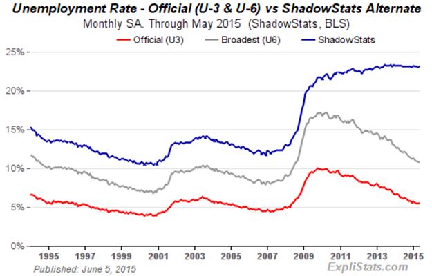
The graph immediately preceding reflects headline May 2015 U.3 unemployment at 5.51%, up from 5.44% in April; headline May U.6 unemployment at 10.79%, versus 10.83% in April; and the headline May ShadowStats unemployment measure at 23.1%, versus 23.0% in April. The ShadowStats-Alternate Unemployment series is built upon the BLS reporting of seasonally-adjusted U.3 and U.6 series, and correspondingly, is affected by the reporting and annual seasonal adjustments to those underlying series.

The following three graphs reflect longer-term unemployment and discouraged-worker conditions. The first graph is of the ShadowStats unemployment measure, with an inverted scale. The higher the unemployment rate, the weaker will be the economy, so the inverted plot tends to move in tandem with plots of most economic statistics, where a lower number means a weaker economy.

The inverted-scale of the ShadowStats unemployment measure also tends to move with the employment-to-population ratio, which is plotted in the second graph (above). Discouraged workers are not counted in the headline labor force, which generally continues to shrink. The labor force containing all unemployed (including total discouraged workers) plus the employed, however, tends to be correlated with the population, so the employment-to-population ratio tends to be something of a surrogate indicator of broad unemployment, and it has a strong correlation with the ShadowStats unemployment measure.

The third graph (above) plots the labor-force participation rate (headline labor force as a percent of population), a series indicated by Federal Reserve Chair Janet Yellen as one she sees as a particularly -good indicator of the health of the labor market. She has mentioned a needed improvement in labor-market health as a precondition for raising interest rates, but such conditions remain under debate. The participation rate was little changed in May 2015, which means, in theory, that the Fed is not about to tighten monetary conditions, if the Fed Chair still is to be believed.

The labor force here is the headline employment plus U.3 unemployment. As with the prior graph of employment-to-population, its holding near a record-low in the current reporting is another indication of problems with long-term discouraged workers, the loss of whom continues to shrink the headline (U.3) labor force, and the plotted ratio. These three graphs reflect detail back to the 1994 redefinitions of the Household Survey. Before 1994, data consistent with May’s reporting simply are not available.

Headline Unemployment Rates. Headline May 2015 unemployment (U.3) increased by 0.07-percentage point to 5.51%, from 5.44% in April. That change is meaningless, though, in the context of the non-comparability of the headline monthly data, which results from the BLS’s reporting methodology and use of concurrent-seasonal-adjustment factors. Those issues are separate from recent official questions raised as to falsification of Current Population Survey results, from which the unemployment detail ultimately is derived (see discussion in Household Survey section of the Reporting Detail).

The headline uptick in the U.3 rate reflected the number of unemployed rising at a faster-proportional pace (by 125,000 or 1.5%), than the increase in the number of employed (by 272,000 or 0.2%), with the labor force increasing by 397,000 or 0.1%. These nonsensical seasonally-adjusted swings may be due to poor-quality seasonal accounting by the BLS as to the initial impact of the end of the school year, but otherwise the numbers are suggestive simply of unusually-large, seasonal-adjustment inconsistencies in the headline monthly comparisons for May 2015.

On an unadjusted basis, the unemployment rates are not revised and at least are consistent in reporting methodology. May’s unadjusted U.3 unemployment rate rose to 5.31%, versus 5.09% in April.

U.6 Unemployment Rate. The broadest unemployment rate published by the BLS, U.6 includes accounting for those marginally attached to the labor force (including short-term discouraged workers) and those who are employed part-time for economic reasons (i.e., they cannot find a full-time job).

With an increase in the underlying seasonally-adjusted U.3 rate, an increase in the adjusted number of people working part-time for economic reasons and a decline in unadjusted discouraged workers and the balance of those marginally attached to the workforce, headline May 2015 U.6 unemployment eased to 10.79%, from 10.83% in April (unchanged at the first-decimal-point reading of 10.8%). The unadjusted U.6 was 10.40% in May, versus 10.36% in April (unchanged at the first-decimal point reading of 10.4%).

ShadowStats Measure. Adding back into the total unemployed and labor force the ShadowStats estimate of the still-growing ranks of excluded, long-term discouraged workers—more in line with common experience—broad unemployment, the May 2015 ShadowStats-Alternate Unemployment Measure, notched higher to 23.1%, versus 23.0% in April and 23.1% in March. Such was down from the 23.3% series high in 2013 (back to 1994). Again, the ShadowStats estimate generally shows the toll of long-term unemployed leaving the headline labor force.

[The Reporting Detail section includes further information on
the employment and unemployment series.]

__________

HYPERINFLATION WATCH

MONETARY CONDITIONS

Broad Money Supply Growth Continued to Slow. Late in 2014, the Federal Reserve ceased net new purchases of U.S. Treasury securities as part of its quantitative easing QE3, but its holdings of Treasury securities have remained stable, near record levels. Despite continued high-level volatility in the monetary base during recent two-week periods, including a record high-level as recently as the period-ended April 15th, annual growth in May 2015 money supply M3 eased back, tentatively to 5.1%, from 5.4% in April and from a recent peak of 5.8% in February. The general monetary circumstance is discussed in No. 692 Special Commentary: 2015 - A World Out of Balance.

Money Supply M3 Annual Growth Tentatively Fell Back to 5.1% in May 2015. Year-to-year growth in May 2015 M3 (ShadowStats-Ongoing Measure) fell back to 5.1%, from 5.4% in April, 5.7% in March and a 68-month high of 5.8% in February 2015, then the strongest showing since June of 2009. Any revisions in the accompanying data generally reflect regular and irregular revisions by the Federal Reserve to the underlying monthly data.

Monthly year-to-year growth in M3 began to slow, after the series hit an interim near-term peak of 4.6% in each of the months of January, February and March 2013, the onset of expanded QE3. Growth then fell to a near-term trough of 3.2% in January 2014, but that period of slowing growth had reversed fully as of May 2014, with annual growth recovering to 4.6%. Annual growth pulled back to 4.4% in June 2014, but rose again to 4.5% in July, easing back to 4.2% in September and October. Growth then jumped to 4.8% and 5.1%, respectively, in November and December 2014, rising to 5.5% in January 2015, and then hitting a five-year high of 5.8% in February. Again, annual growth has been falling off since February, hitting 5.1% in May.

Formal M3 estimates and the first readings of annual growth for M2 and M1 in May 2015 will be updated on the Alternate Data tab of www.ShadowStats.com by June 6th.

The seasonally-adjusted, early estimate of month-to-month change for May 2015 money supply M3 was roughly a gain 0.2%, versus an unrevised gain of 0.1% in April 2015. Estimated month-to-month M3 changes, however, remain less reliable than are the estimates of annual growth.

Growth for March M1 and M2. For May 2015, year-to-year and month-to-month changes follow for the narrower M1 and M2 measures (M2 includes M1; M3 includes M2). See the Money Supply Special Report for full definitions of those measures.

Annual M2 growth in May 2015 slowed to 5.8%, from 6.0% in April, with a month-to-month gain of about 0.3% in May, versus 0.4% in April. For M1, year-to-year growth slowed to an initial estimate of 7.3% in May 2015, versus a revised 8.1% (previously 7.8%) gain in April 2015, with a month-to-month contraction of 0.2% (-0.2%) in May 2015, versus a revised gain of 0.2% (previously unchanged) in April.

With the Monetary Base Oscillating Near a Record High, "Quantitative Easing" Remains in Play, Symptomatic of the Fed Having Lost Control? Discussed in No. 692 Special Commentary: 2015 - A World Out of Balance, the Fed’s primary mission is to keep the banking system solvent and afloat, but that was not working, coming into the Panic of 2008. Quantitative easing was introduced in 2008 and went through a number of phases, as reflected in the size of, and growth in the monetary base shown in the accompanying graphs. Where normally such growth would have translated into extraordinary growth in the money supply, it has not. Only as the Fed has pulled back from aggressive assets purchases did M3 begun to show a little, temporary upside movement.

The extraordinary level of asset purchases by the Fed did not flow through to the broad economy, because banks did not lend into the normal flow of commerce, and there was no resulting significant upside movement in money supply, as a result. Instead, banks turned the funds back to the Fed as excess reserves, earning interest and providing support to the stock market. As part of this process, the Fed ended up monetizing the bulk of the U.S. Treasury’s funding needs during the period of active buying, paying back interest earned on the securities to the Treasury.

With the Fed having ceased purchases of new Treasury securities late in 2014 (maturing issues still are rolled over), the monetary base has continued its recent pattern of volatility at high-levels. Having set a record high level of $4.167 trillion in the two-week period ended April 15, 2015, the monetary base (Saint Louis Fed measure) backed off in the latest three bi-weekly periods, ended May 27th, with an average $3.951 billion in the latest period. This pattern of high-level fluctuation has been common since the Fed ended its active purchasing of net new assets.

The Fed’s Treasury asset holdings effectively have continued at or near an all-time high, in the context of ongoing QE3. The expressed desire by some in the Fed to push interest rates higher, to more-normal levels, combined with a failing economy that should provide a practical restraint to such action, is suggestive of an economic-and-monetary system that has moved beyond effective control of the U.S. central bank and the federal government, as discussed in the Opening Comments.

__________

REPORTING DETAIL

EMPLOYMENT AND UNEMPLOYMENT (May 2015)

Seasonal-Factor Distortions Significantly Skewed May Labor Data. [Through the Payroll Survey Detail, this section, largely repeats material in the Opening Comments.] Headline May 2015 payrolls jumped by a stronger-than-expected 280,000 jobs, and the level of April payrolls revised higher by 32,000. Yet, the bulk of the excess employment gain was due to the non-comparable, inconsistent and unpublished shifting of seasonal-adjustment factors, not due to resurgent economic activity. The minor increase in headline U.3 unemployment from 5.4% to 5.5% was without any significance.

From the Establishment Survey, consider that the unadjusted level of April 2015 payrolls revised lower by 12,000, but the seasonally-adjusted level revised higher by 32,000. The positive swing of 44,000 jobs was due primarily to the monthly revamping of seasonal adjustments, which accompanies the headline monthly payroll calculation, and which boosted the apparent headline growth in April and setting up the bigger-than -expected May gain. The seasonal-adjustment shifting can be seen in the graph in the Headline Distortions from Shifting Concurrent Seasonal Factors section. If the regular monthly seasonals were reasonably honest, all those lines would be close to flat, near zero.

PAYROLL SURVEY DETAIL. The Bureau of Labor Statistics (BLS) published the headline employment and unemployment data for May 2105, today, June 5th. In the context of seasonally-warped upside revisions to the headline levels of March and April payrolls, the seasonally-adjusted, headline gain for May was 280,000 jobs +/- 129,000 (95% confidence interval). Net of prior-period revisions, the gain in May payroll employment was 312,000 jobs.

The 280,000 jump in payrolls followed a downwardly-revised gain of 221,000 [previously 223,000] in April, and an upwardly-revised (but deliberately-overstated) gain of 119,000 [previously up by 85,000, initially up by 125,000] in March.

Inconsistent, Non-Comparable and Deliberately-Misstated Monthly Gains for March 2015 and Before. Headline monthly payroll detail is not comparable with earlier months, back more than one month from the headline month, due to the BLS’s misuse of concurrent-seasonal-factor adjustments. Discussed in the later Headline Distortions from Shifting Concurrent Seasonal Factors section, the reporting fraud comes not from the adjustment process, itself, but rather from the Bureau deliberately not publishing a consistent headline history, where a new history is generated and available each month, along with the recalculation of the seasonal factors unique to creating the current month’s headline detail.

As a result, the headline 280,000 monthly gain in May 2015 payrolls was inconsistent with and not comparable to the headline revised March 2015 gain of 119,000 [previously up by 85,000]. The gain consistent with the new headline May detail was 107,000 for March, some 12,000 less than the official number. Such was a planned and regular misstatement of headline payroll activity by the BLS.

Headline differences can be more significant. For example, the headline monthly gain for November 2014 payrolls still is 423,000, but that never was true. That number came out of the 2014 benchmark reporting, including headline January 2015, but the November change versus October—consistent with the headline reporting of the time—was 337,000, some 86,000 less. With intervening monthly revisions, and now consistent with headline May 2015 reporting and recalculations, the aggregate November and October levels have changed some, but the November 2014 versus October 2014 gain coincidently still remained 86,000 less than the headline 423,000 in the latest detail. The consistent and comparable historical numbers change each month, with the consistent series explored fully in Commentary No. 695.

“Trend Model” for June 2015 Headline Payroll-Employment Change. Discussed in Commentary No. 717, and as described generally in Payroll Trends, the trend indication from the BLS’s concurrent-seasonal-adjustment model—prepared by our affiliate www.ExpliStats.com—was for a May 2015 monthly payroll gain of 214,000, based on the BLS trend model structured into the actual headline reporting of April 2015. Consensus estimates tend to settle around the trend, where late-consensus expectations for May 2015 ranged from 210,000 [MarketWatch] to 220,000 [Bloomberg]. The 280,000-headline gain topped both the trend and consensus estimates. Although not the case in the current circumstance, reporting surprises sometimes are signaled, in the direction of the trend, when there are sharp variations between the trend and consensus expectations.

June 2015 Trend Estimate. Exclusive to ShadowStats subscribers, based on May 2015 reporting, the ExpliStats trend number calculations suggest a BLS-based headline gain of 236,000 for June 2015. That is the level around which the June consensus expectations should settle.

Confidence Intervals. Where the current employment levels have been spiked by misleading and inconsistently-reported concurrent-seasonal-factor adjustments, the reporting issues suggest that a 95% confidence interval around the modeling of the monthly headline payroll gain should be well in excess of +/- 200,000, instead of the official +/- 129,000. Even if the data were reported on a comparable month-to-month basis, other reporting issues would prevent the indicated headline magnitudes of change from being significant. Encompassing Birth-Death Model biases, the confidence interval more appropriately should be in excess of +/- 300,000.

May Construction-Payroll Growth in Context of Downside Revisions to April. The accompanying graph of construction-payroll employment updates the plot of the April detail shown in prior Commentary No. 724 covering April 2015 construction spending.

On top of heavy downside revisions to the levels of activity in March and April, headline May 2015 construction payrolls came in at 6.387 million jobs. That was up by 17,000 from the revised April 2015 level but up by just 4,000, net of the prior-period revisions. The April 2015 detail reflected a revised monthly gain of 35,000 [previously up by 45,000], versus a revised March decline of 12,000 (-12,000) [previously down by 9,000 (-9,000), initially down by 1,000 (-1,000)] jobs versus February.

The ongoing relative strong growth in headline construction jobs, albeit slower in revision, ran counter to all other indications of flat-to-down construction activity, up through March. Yet, headline activity in the unstable headline-monthly reporting of housing starts and construction spending picked up sharply in April. Those numbers likely will revise lower, along with the construction jobs. Construction-payroll numbers remain heavily biased to the upside (officially bloated by 6,000 jobs per month, unofficially at an order of magnitude of 20,000 jobs per month). Nonetheless, total May 2015 construction jobs were down by 17.4% (-17.4%) from the April 2006 pre-recession peak for the series.

Historical Payroll Levels. Payroll employment is a coincident indicator of economic activity, and irrespective of all the reporting issues with the series, payroll employment formally regained its pre-recession high in 2014, despite the GDP purportedly having done the same three years earlier, back in 2011. Reflected in the next two graphs, headline payroll employment moved to above its pre-recession high in April 2014 (it had happened in May 2014 pre-benchmarking), and it has continued to rise, now about 3.0 million jobs above the pre-recession peak.

The first two graphs show the headline payroll series, both on a shorter-term basis, since 2000, and on a longer-term historical basis, from 1940. In perspective, the longer-term graph of the headline payroll-employment levels shows the extreme duration of what had been the official non-recovery in payrolls, the worst such circumstance of the post-Great Depression era.

Beyond excessive upside add-factor biases built into the monthly calculations (see the Birth-Death Model section), the problem remains that payroll employment counts the number of jobs, not the number of people who are employed. Much of that payroll "jobs" growth is in multiple part-time jobs, many taken on for economic reasons, where full-time employment was desired but could not be found.

Full-Time Employment versus Part-Time Payroll Jobs. Shown in the accompanying graph, as of May 2015, the level of full-time employment—from the Household Survey—still was 0.8 million shy of its precession high, purportedly having rebounded by 630,000 in May 2015, having declined by in April by 252,000 (-252,000). Headline month-to-month volatility here is more a function of the instabilities from non-comparability of the monthly data (see the discussion in the Headline Distortions from Shifting Concurrent Seasonal Factors section), as opposed to month-to-month volatility in economic activity.

As an aside, that shortfall would be even greater, except for the regular annual games the BLS plays with its "population adjustments." ShadowStats continues to work on an alternate measure for the employment numbers from both the Household and Payroll Series. More will be forthcoming on this.

The graph of full-time employment excludes the count of those employed with one-or-more part-time jobs. Total employment, including those employed with part-time work, also has recovered its pre-recession high, but still not close to the payroll reporting. Again, the Household Survey numbers count the number of people who have at least one job. The Payroll Survey simply counts the number of jobs (see Commentary No. 686 for further detail).

Annual Percent Change in Payrolls—Growth Down from Near-Term Peak. Not-seasonally-adjusted, year-to-year change in payroll employment is untouched by the concurrent-seasonal-adjustment issues, so the monthly comparisons of year-to-year change at least are reported on a consistent basis. Yet, a possible new redefinition of the series—not the standard benchmarking process in 2014—appears to be in play, on top of the prior distortions from the 2013 benchmarking (see Commentary No. 598).

With bottom-bouncing patterns of recent years, current headline annual growth has recovered from the post-World War II record 5.02% (-5.02%) decline seen in August 2009, as shown in the accompanying graphs. That 5.02% (-5.02%) decline remains the most severe annual contraction since the production shutdown at the end of World War II [a trough of a 7.59% (-7.59%) annual contraction in September 1945]. Disallowing the post-war shutdown as a normal business cycle, the August 2009 annual decline was the worst since the Great Depression.

Headline Distortions from Shifting Concurrent Seasonal Factors. Detailed in Commentary No. 694 and Commentary No. 695, there are serious and deliberate reporting flaws with the government’s seasonally-adjusted, monthly reporting of both employment and unemployment. Each month, the BLS uses a concurrent-seasonal-adjustment process to adjust both the payroll and unemployment data for the latest seasonal patterns. As new headline data are seasonally-adjusted for each series, the re-adjustment process also revises the monthly history of each series, recalculating prior, adjusted reporting for every month, going back five years, so as to be consistent with the new seasonal patterns that generated the current headline number.

Effective Reporting Fraud. The problem is that the BLS does not publish the monthly historical revisions along with the new headline data. As a result, current headline reporting is neither consistent nor comparable with prior data, and the unreported actual monthly variations versus headline detail can be large. The deliberately-misleading reporting effectively is a fraud. The problem is not with the BLS using concurrent-seasonal-adjustment factors, it is with the BLS not publishing consistent data, where those data are calculated each month and are available internally to the Bureau.

Household Survey. In the case of the published Household Survey (unemployment rate and related data), the seasonally-adjusted headline May 2015 numbers are not comparable with the headline April 2015 data or any month before. Accordingly, the published headline detail as to whether the unemployment rate was up, down or unchanged in a given month is not meaningful, and what actually happened is not knowable by the public. Month-to-month comparisons of these popular numbers are of no substance, other than for market hyping or political propaganda.

The headline month-to-month reporting is made consistent in the once-per-year reporting of December data, when the annual revisions to the faux "fixed" seasonal adjustments are published. All historical comparability evaporates, though, with the ensuing month’s headline January reporting, and with each monthly estimate thereafter.

Payroll or Establishment Survey. In the case of the published Payroll Survey data (payroll-employment change and related detail), monthly changes in the seasonally-adjusted headline May 2015 data are comparable only with the headline changes in the April 2015 numbers, not with March 2015 or any earlier months. Due to the BLS modeling process, the historical data never are published on a consistent basis, even with publication of the annual benchmark revision, as discussed shortly.

No one seems to mind if the published earlier numbers are wrong, particularly if unstable seasonal-adjustment patterns have shifted prior jobs growth or reduced unemployment into current reporting, as often is the case, without any formal indication of the shift from the previously-published historical data.

The BLS does provide modeling detail for the Payroll Survey, allowing for third-party calculations, but no such accommodation has been made for the Household Survey. ShadowStats affiliate ExpliStats does such third-party calculations, and the detail of the differences between the current headline reporting and the constantly-shifting, consistent and comparable history are plotted in the accompanying graph.

The preceding chart details how far the monthly payroll employment data have strayed from being consistent with the most recent benchmark revision. The gray line shows that December 2014 pattern versus the 2013-benchmark revision, and the color-coded lines show the January to May 2015 patterns of distortion versus the 2014-benchmark. Due to several months of testing of the model, before the benchmark release, the BLS never publishes the historical data on a consistent basis.

A comparison of the heavy, dark-blue line (May 2015) with the thin orange line (April 2015), shows the positive, one-month shift in seasonal factors that boosted the revised headline reporting of the adjusted March and April reporting. That now overstated adjusted March level will remain in the base data until February 2016.

If the headline reporting were comparable and stable, month-after-month, all the lines in the graph would be flat and at zero. Here, with the payroll series, again, only the headline month and the prior month are consistent in terms of month-to-month reporting detail (headline March 2015 detail no longer is consistent nor comparable with data from February 2015 or earlier. It is overstated by 12,000 jobs, as discussed in the earlier section Inconsistent, Non-Comparable and Deliberately-Misstated Monthly Gains.

Birth-Death/Bias-Factor Adjustment. Despite the ongoing, general overstatement of monthly payroll employment, the BLS adds in upside monthly biases to the payroll employment numbers. The continual overstatement is evidenced usually by regular and massive, annual downward benchmark revisions (2011 and 2012 and 2014 excepted). As discussed in the benchmark detail of Commentary No. 598, the regular benchmark revision to March 2013 payroll employment was to the downside by 119,000, where the BLS had overestimated standard payroll employment growth.

With the March 2013 revision, though, the BLS separately redefined the Payroll Survey so as to include 466,000 workers who had been in a category not previously counted in payroll employment. The latter event was little more than a gimmicked, upside fudge-factor, used to mask the effects of the regular downside revisions to employment surveying, and likely is the excuse behind the increase in the annual bias factor, where the new category cannot be surveyed easily or regularly by the BLS. Elements tied to this likely had impact on the unusual issues with the 2014 benchmark revisions.

Abuses from the 2014 benchmarking are detailed in Commentary No. 694 and Commentary No. 695. With the headline benchmark revision for March 2014 showing a jobs understatement of 67,000, the BLS upped its annual add-factor bias by an even greater 161,000 for the year ahead, to 892,000. As has been standard BLS practice, there is no good political reason for risking a headline understatement of jobs growth.

Historically, the upside-bias process was created simply by adding in a monthly "bias factor," so as to prevent the otherwise potential political embarrassment to the BLS of understating monthly jobs growth. The "bias factor" process resulted from such an actual embarrassment, with the underestimation of jobs growth coming out of the 1983 recession. That process eventually was recast as the now infamous Birth-Death Model (BDM), which purportedly models the effects of new business creation versus existing business bankruptcies.

May 2015 Add-Factor Bias. The not-seasonally-adjusted May 2015 bias was a positive monthly add-factor of 213,000, the same as the positive monthly add-factor of 213,000 in April 2015, and versus a positive monthly add-factor of 204,000 in May 2014. The BLS has begun quarterly revisions to the biases, and the first cut seems to indicate something of a slowing pace of upside biases, versus prior reporting, coincident with what still appears otherwise to be a broad slowing in economic activity. Such a shift would mean that first-quarter 2015 jobs growth likely was overstated as seen internally in official calculations.

The revamped, aggregate upside bias for the trailing twelve months through May 2015 was 856,000, versus 847,000 in of April 2015, and versus the pre-benchmarked level of 731,000 in December 2014. That was an unchanged rough-monthly average of 71,000 in May and April (versus 61,000 pre-benchmark) jobs created out of thin air, on top of some indeterminable amount of other jobs that are lost in the economy from business closings. Those losses simply are assumed away by the BLS in the BDM, as discussed below.

Problems with the Model. The aggregated upside annual reporting bias in the BDM reflects an ongoing assumption of a net positive jobs creation by new companies versus those going out of business. Such becomes a self-fulfilling system, as the upside biases boost reporting for financial-market and political needs, with relatively good headline data, while often also setting up downside benchmark revisions for the next year, which traditionally are ignored by the media and the politicians. The BLS cannot measure meaningfully the impact of jobs loss and jobs creation from employers starting up or going out of business, on a timely basis (within at least five years, if ever), or by changes in household employment that were incorporated into the 2014 redefined payroll series. Such information simply is guesstimated by the BLS, along with the addition of a bias-factor generated by the BDM.

Positive assumptions—commonly built into government statistical reporting and modeling—tend to result in overstated official estimates of general economic growth. Along with these happy guesstimates, there usually are underlying assumptions of perpetual economic growth in most models. Accordingly, the functioning and relevance of those models become impaired during periods of economic downturn, and the current, ongoing downturn has been the most severe—in depth as well as duration—since the Great Depression.

Indeed, historically, the BDM biases have tended to overstate payroll employment levels—to understate employment declines—during recessions. There is a faulty underlying premise here that jobs created by start-up companies in this downturn have more than offset jobs lost by companies going out of business. Recent studies have suggested that there is a net jobs loss, not gain, in this circumstance. So, if a company fails to report its payrolls because it has gone out of business (or has been devastated by a hurricane), the BLS assumes the firm still has its previously-reported employees and adjusts those numbers for the trend in the company’s industry.

Further, the presumed net additional “surplus” jobs created by start-up firms are added on to the payroll estimates each month as a special add-factor. These add-factors are set now to add an average of 71,000 jobs per month in the current year. In current reporting, the aggregate average overstatement of employment change easily exceeds 200,000 jobs per month.

HOUSEHOLD SURVEY DETAIL. Discussed in the earlier Headline Distortions from Shifting Concurrent Seasonal Factors section, seasonally-adjusted data from the monthly Household Survey simply are not comparable on a month-to-month basis. In this form, headline monthly changes in the unemployment-related numbers are virtually meaningless, good only for the market- or political-hype of the moment. The seasonal-adjustment process here restates the history of each series, each month, as unique adjustment factors determine the current month’s headline detail. Yet, when the BLS publishes the headline numbers, it does not publish the comparable revised history. Only the BLS, not the public, knows the actual, comparable monthly change in the seasonally-adjusted U.3-unemployment rate.

Separately, detailed in Commentary No. 669, significant issues as to falsification of the data gathered in the monthly Current Population Survey (CPS), conducted by the Census Bureau, have been raised in the press and investigated by the House Committee on Oversight and Government Reform and the U.S. Congress Joint Economic Committee. Further investigation purportedly is underway with the new Congress. CPS is the source of the Household Survey used by the BLS in estimating monthly unemployment, employment, etc. Accordingly, the statistical significance of the headline reporting detail here is open to serious question.

Headline Unemployment Rates. The headline May 2015 unemployment (U.3) rate increased by 0.07-percentage point to 5.51%, from 5.44% in April. Technically, the headline May gain in U.3 was statistically-insignificant, where the official 95% confidence interval around the monthly change in headline U.3 is +/- 0.23-percentage point. That is meaningless, though, in the context of the comparative month-to-month reporting-inconsistencies created by the concurrent-seasonal factors, let alone new questions as to general survey accuracy and significance.

The headline uptick in the U.3 rate reflected the number of unemployed rising at a faster-proportional pace (by 125,000 or 1.5%), than the increase in the number of employed (by 272,000 or 0.2%), with the labor force increasing by 397,000 or 0.1%. The data were nonsensical in various elements, suggesting unusually-large, seasonal-adjustment inconsistencies in the headline monthly comparisons for May 2015. Such could become evident with the benchmark reporting, due in conjunction with headline December 2015 detail, to be published in January 2016.

On an unadjusted basis, the unemployment rates are not revised and at least are consistent in reporting methodology. May’s unadjusted U.3 unemployment rate rose to 5.31%, versus 5.09% in April.

New discouraged workers always are moving into U.6 unemployment accounting from U.3, while those who have been discouraged for one year continuously are dropped from the U.6 measure. As a result, the U.6 measure has been easing along with U.3, for a while, but those being pushed out of U.6 still are counted in the ShadowStats Alternate Unemployment Measure, which generally has remained stable.

"Short-Term" Discouraged Workers. The count of short-term discouraged workers in May 2015 (never seasonally-adjusted) dropped to 563,000 from 756,000 in April, and versus 738,000 in March. The latest, official discouraged-worker number reflected the flow of the unemployed—giving up looking for work—leaving the headline U.3 unemployment category and being rolled into the U.6 measure as short-term “discouraged workers,” net of the further increase in the number of those moving from short-term discouraged-worker status into the netherworld of long-term discouraged-worker status.

It is the long-term discouraged-worker category that defines the ShadowStats-Alternate Unemployment Measure. There is a relatively heavy, continuing rollover from the short-term to the long-term category, with the ShadowStats measure encompassing U.6 and the short-term discouraged workers, plus the long-term discouraged workers. In 1994, “discouraged workers”—those who had given up looking for a job because there were no jobs to be had—were redefined so as to be counted only if they had been “discouraged” for less than a year. This time qualification defined away a large number of long-term discouraged workers. The remaining short-term discouraged workers were included in U.6.

ShadowStats-Alternate Unemployment Rate Measure. Adding back into the total unemployed and labor force the ShadowStats estimate of the still-growing ranks of excluded, long-term discouraged workers—more in line with common experience—broad unemployment, the May 2015 ShadowStats-Alternate Unemployment Measure notched higher, back to 23.1%, versus 23.0% in April 23.0% and 23.1% in March. That was down from the 23.3% series high in 2013 (back to 1994).

The ShadowStats-Alternate estimate reflects the toll of the long-term unemployed leaving the headline labor force. Where the ShadowStats estimate generally is built on top of the official U.6 reporting, it tends to follow its relative monthly movements and particularly its annual revisions. Accordingly, the alternate measure often will suffer some of the same seasonal-adjustment woes that afflict the base series, again, including underlying annual revisions.

The ShadowStats estimates of long-term discouraged workers reflect a proprietary analysis of the flows of discouraged workers, including attrition, developed using government and private surveying in the two decades since the 1994 overhaul of the unemployment surveying.

[The remaining text in this section is unchanged from the prior Commentary.] As seen in the usual graph of the various unemployment measures (in the Opening Comments), there continues to be a noticeable divergence in the ShadowStats series versus U.6, and the ShadowStats series and U.6 versus U.3. The reason for this is that U.6, again, only includes discouraged workers who have been discouraged for less than a year. As the discouraged-worker status ages, those that go beyond one year fall off the government counting, even as new workers enter “discouraged” status. A similar pattern of U.3 unemployed becoming “discouraged” and moving into the U.6 category also accounts for the early divergence between the U.6 and U.3 categories.

With the continual rollover, the flow of headline workers continues into the short-term discouraged workers category (U.6), and from U.6 into long-term discouraged worker status (a ShadowStats measure). There was a lag in this happening as those having difficulty during the early months of the economic collapse, first moved into short-term discouraged status, and then, a year later into long–term discouraged status, hence the lack of earlier divergence between the series. The movement of the discouraged unemployed out of the headline labor force has been accelerating. While there is attrition in long-term discouraged numbers, there is no set cut off where the long-term discouraged workers cease to exist. See the Alternate Data tab for historical detail.

Generally, where the U.6 largely encompasses U.3, the ShadowStats measure encompasses U.6. To the extent that a decline in U.3 reflects unemployed moving into U.6, or a decline in U.6 reflects short-term discouraged workers moving into the ShadowStats number, the ShadowStats number continues to encompass all the unemployed, irrespective of the series from which they otherwise may have been ejected.

Three further related graphs, also found in the Opening Comments section, are of the ShadowStats-Alternate Unemployment Measure, with an inverted scale, the employment-to-population ratio, which has a high correlation with the inverted ShadowStats measure, and participation rate, a measure commonly touted by Federal Reserve Chair Janet Yellen.

Great Depression Comparisons. As discussed in the regular Commentaries covering the monthly unemployment circumstance, an unemployment rate around 23% might raise questions in terms of a comparison with the purported peak unemployment in the Great Depression (1933) of 25%. Hard estimates of the ShadowStats series are difficult to generate on a regular monthly basis before 1994, given the reporting inconsistencies created by the BLS when it revamped unemployment reporting at that time. Nonetheless, as best estimated, the current ShadowStats level likely is about as bad as the peak actual unemployment seen in the 1973-to-1975 recession and in the double-dip recession of the early-1980s.

The Great Depression unemployment rate of 25% was estimated well after the fact, with 27% of those employed working on farms. Today, less than 2% of the employed work on farms. Accordingly, a better measure for comparison with the ShadowStats number would be the Great Depression peak in the nonfarm unemployment rate in 1933 of roughly 34% to 35%.

__________

WEEK AHEAD

Headline Economic Reporting and Revisions Should Trend Much Weaker versus Overly-Optimistic Expectations; Inflation Will Rise Anew, Along with Rising Oil Prices. In a fluctuating trend to the downside, amidst still-predominantly-negative reporting and surprises in headline numbers, market expectations for business activity nonetheless respond to the latest market hype. The general effect tends to hold the market outlook at overly-optimistic levels. Expectations exceed any potential, underlying economic reality.

GDP excesses from 2014 should face downside adjustments in the July 30, 2015 GDP benchmark revision, and expectations for headline growth estimates of, or further revisions to first- and second-quarter 2015 should continue shifting to the downside, increasingly into negative territory, shy of upside-jawboning of the data in the press, as discussed in the Opening Comments of Commentary No. 722.

Headline CPI-U consumer inflation—recently driven lower by collapsing prices for gasoline and other oil-price related commodities—likely is close to its near-term, year-to-year low, having shown monthly declines in annual inflation of less than a full 0.1% (-0.1%) in the three months through March 2015, but dropping by 0.2% (-0.2%) in April 2015. A large jump in gasoline prices for May 2015 and a softening of negative seasonal-adjustments for gasoline promise a headline increase in May 2015 CPI-U inflation, with annual inflation likely pulling at least even with zero.

Significant upside inflation pressures are building, as oil prices rebound, a process that should accelerate rapidly with the eventual sharp downturn in the exchange-rate value of the U.S. dollar. These areas, the general economic outlook and longer range reporting trends are reviewed broadly in No. 692 Special Commentary: 2015 - A World Out of Balance.

A Note on Reporting-Quality Issues and Systemic-Reporting Biases. Significant reporting-quality problems remain with most major economic series. Again, see the Commentary No. 722 as to current market and political pressures on the Bureau of Economic Analysis (BEA) relative to GDP reporting. Any meaningful, overt shifts by the BEA in headline GDP reporting methodology, other than those already planned for the July 30, 2015 benchmarking, would be extraordinary in terms of BEA behavior and are not likely. Still, some gimmicked, less-negative summary numbers already have been planned for publication.

Beyond the pre-announced gimmicked changes to reporting methodologies of the last several decades, ongoing headline reporting issues are tied largely to systemic distortions of monthly seasonal adjustments. Data instabilities were induced partially by the still-evolving economic turmoil of the last eight years, which has been without precedent in the post-World War II era of modern-economic reporting. The severity and ongoing nature of the downturn provide particularly unstable headline economic results, when concurrent seasonal adjustments are used (as with retail sales, durable goods orders, employment and unemployment data, explored in the labor-data related Commentary No. 695).

Combined with recent allegations of Census Bureau falsification of data in its monthly Current Population Survey (the source for the Bureau of Labor Statistics’ Household Survey), these issues have thrown into question the statistical-significance of the headline month-to-month reporting for many popular economic series (see Commentary No. 669).

PENDING RELEASES:

Nominal Retail Sales (May 2015). The Census Bureau has scheduled release of May 2015 nominal (not-adjusted-for-inflation) retail sales for Thursday, June 11th. Real (inflation-adjusted) retail sales for May will be published in ShadowStats Commentary No. 729 of June 18th, in conjunction with the detail on headline CPI-U reporting for May. Early expectations appear to be for a big headline jump for the nominal retail series, following headline "unchanged" activity in April. MarketWatch indicates expectations for a 1.0% monthly gain.

With this series, though, and in this environment, downside-reporting surprises usually are a good bet, including a weaker-than-expected headline number and potential downside revisions to the March and April headline data.

Net of inflation adjustment, real retail sales in May likely will have contracted again, helping to set the stage for a second consecutive quarterly decline with second-quarter 2015 GDP, following on top of the headline first-quarter GDP contraction.

Constraining sales activity, the consumer remains in an extreme liquidity bind, as updated most recently in Commentary No. 723, and as discussed in No. 692 Special Commentary: 2015 - A World Out of Balance. Without sustained growth in real income, and without the ability and/or willingness to take on meaningful new debt in order to make up for the income shortfall, the U.S. consumer is unable to sustain positive growth in domestic personal consumption, including retail sales, real or otherwise.

Producer Price Index—PPI (May 2015). The Bureau of Labor Statistics (BLS) will release the May 2015 PPI on Friday, June 12th. ShadowStats Commentary No. 727 of June 15th will discuss the detail. Early-consensus expectations are for a sharp pick-up in May wholesale inflation, with MarketWatch indicating an expected, headline monthly gain of 0.6%, versus the current headline April PPI contraction of 0.4% (-0.4%).

Expectations for a strong increase are reasonable, given rising energy inflation and positive shifts in related seasonal factors. A major constraint on headline-PPI inflation, however, is the perverse, reverse-inflation impact that rising costs have in the now-dominant services sector. Although indicating future inflationary pressures, rapidly-rising costs tend to reduce near-term service-sector margins, a circumstance that is deflationary, per BLS definition.

While the collapse in oil and gasoline prices bottomed out in February 2015, pricing pressures were mixed in March (oil down, gasoline up) but generally rose in April. Yet, the headline, seasonally-unadjusted energy numbers fell in the April PPI, before negative seasonal-adjustments exaggerated the inflation understatement.

Unadjusted energy prices rose sharply again in May. Based on the two most-widely-followed oil contracts, not-seasonally-adjusted, monthly-average oil prices gained 7.7% and 9.9% for the month, with an accompanying increase of 9.7% in unadjusted monthly-average retail-gasoline prices (Department of Energy). Further, PPI seasonal adjustments for energy costs turn positive in May.

While catch-up reporting and positive seasonal shifts should boost headline PPI inflation, again, the inverse-inflation reaction of shifting oil prices in the services sector is nonsensically offsetting. Where rising oil prices also are reflected usually in near-term falling margins (service-sector deflation), such should mute somewhat the energy-related inflation boost that otherwise would and should dominate the headline May PPI.

Along with added monthly inflation from wholesale food and “core” goods (everything but food and energy), a fair gain in the headline PPI still is a reasonable expectation.

__________