COMMENTARY NUMBER 572
October Employment and Unemployment

November 8, 2013

__________

Large Shift in August-October Period Seasonal Adjustments
Bloated Latest Payroll Reporting

Loss of Long-Term Unemployed from Headline Labor Force
Boosted Alternate Unemployment Rate to New High

Government-Shutdown Impact on October Unemployment Reporting
Masked by Misclassification and Seasonal-Adjustment Fiasco

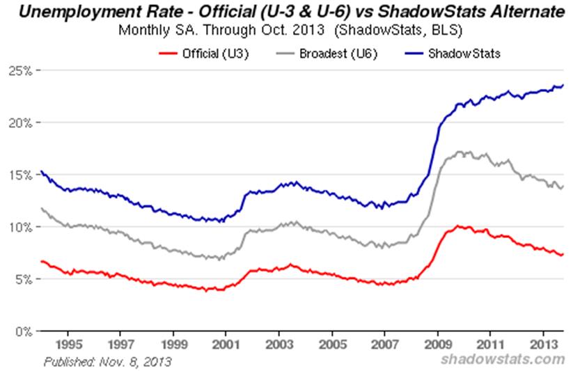
October Unemployment: 7.3% (U.3), 13.8% (U.6), 23.5% (ShadowStats)
__________

 

PLEASE NOTE: The next regular Commentary is scheduled for Friday, November 15th, covering October industrial production and the September trade balance.

Best wishes to all — John Williams

 

OPENING COMMENTS AND EXECUTIVE SUMMARY

With Washington awash in scandals, political turmoil and sinking approval ratings, the political timing could not have been better for this morning’s (November 8th) stronger-than-expected jobs report from the Bureau of Labor Statistics (BLS).  An unusual shift of favorable seasonal-adjustment factors—into the August, September and October reporting period—boosted the latest jobs numbers.  The jobs growth borrowed from other periods will be buried in the next benchmark revision or will be re-shifted in the months ahead, with the details never to surface in official reporting.  Separately, the October payroll survey counted furloughed government employees as employed, as the BLS previously had indicated.

On the unemployment front, however, the household survey was to count furloughed employees as unemployed, but half of those unemployed government workers were misclassified and were counted instead as employed.  While BLS recognizes the error, it will not correct it.  At the same time, the increase in unemployment—from those who were counted—helped to mask a decline in longer-term unemployed, who were moved out of the headline labor force.

The general economic outlook here has not changed a bit.  The current labor reporting is just not to be believed.  Given the special nature of October’s employment and unemployment reporting issues, these Opening Comments will cover the broad picture of the labor releases, with the Reporting Detail section covering primarily the hard numbers and the usual updates to other reporting-quality issues.  The headline October household survey data, however, are worthless.

The latest details on consumer credit (September) and consumer sentiment (early-November) are plotted in graphs at the end of the Opening Comments section.  There has been no improvement in the liquidity issues constraining consumer spending, while consumer sentiment still is in deterioration and at a level that historically only has been seen during recessions.

The initial estimate of year-to-year growth in the ShadowStats-Ongoing M3 Measure for October 2013 normally would be published with this Commentary, and an increase in annual growth is likely.  As noted in the Hyperinflation Watch section, however, due to unusually-high volatility in the weekly data used in putting together the M3 estimate, the publication of the detail will be over the weekend (November 9th) on the Alternate Data tab of www.ShadowStats.com.  A brief Commentary on the latest money supply numbers will follow early in the week ahead.

 

Scrambled Unemployment and Employment Data.  Irrespective of the mixed-up unemployment reporting, keep in mind that distortions from the government shutdown and partial counting of furloughed employees as unemployed will reverse out in November’s reporting.  The big story out of the October household survey was the 720,000 decline in the headline labor force, which largely reflected the loss of longer-term unemployed into the broader U-6 and ShadowStats unemployment measures.

The use of concurrent seasonal factors (see the section by the same name in the Reporting Detail), and the practice of reporting headline payroll-employment change and revisions for just two months, allowed for a massive shift in seasonal factors to boost the latest jobs reporting.  As will be discussed, for example, the headline monthly jobs gain in August 2013 was revised (inflated) to 238,000 from prior reporting of 193,000, but August and July detail—as of October—no longer were reported officially on a comparable basis.  The comparable August gain versus July was 206,000.  Based on the BLS’s consistent but unpublished reporting, which is estimated privately by ShadowStats—using BLS detail and models—the August gain actually was 32,000 less than the official reporting, much closer to the prior growth estimate.

October Unemployment Reporting Issues related to Furloughed Government Employees.  The grievous misreporting by the BLS of the impact of the government shutdown on the headline October 2013 unemployment rate (U.3) is illustrative of serious issues within the BLS surveying and reporting, and what well may be political considerations as to how the data were handled.  Again, whatever is the impact on October U.3 unemployment from the furloughed government employees, those distortions should reverse with November’s reporting.

The headline U.3 unemployment rate was 7.3% in October, up from 7.2% in September.  Without the limited portion of the furloughed employees counted as unemployed by the BLS, the headline U.3 would have dropped to about 7.1% in October, reflecting a large loss of longer-term unemployed moving out of the headline labor force.  If the full 400,000 furloughed workers who were counted by the BLS had been included, headline October unemployment would have risen to about 7.4%.  So, in summary, versus a headline September 7.2% for U.3, the headline October U.3 would have been 7.1% without considering the government shutdown.  It was a headline 7.3%, as reported, but with misclassifications of the unemployed.  It would have been 7.4% including full furlough impact.  Separately of course, due to the same concurrent seasonal factor adjustments that warp the payroll reporting, the headline September and October numbers would not have comparable in any of those circumstances, anyway (again, see the concurrent seasonal factor section in the Reporting Detail).

Here are the BLS explanations from their press release of today, as to what happened with the government furloughs [and some ShadowStats observations]:

“Both the number of unemployed persons, at 11.3 million, and the unemployment rate, at 7.3 percent, changed little in October [number of unemployed rose by just 17,000].  Among the unemployed, however, the number who reported being on temporary layoff increased by 448,000.  This figure includes furloughed federal employees [204,000 unadjusted were furloughed workers] who were classified as unemployed on temporary layoff under the definitions used in the household survey.  (Estimates of the unemployed by reason, such as temporary layoff and job leavers, do not sum to the official seasonally adjusted measure of total unemployed because they are independently seasonally adjusted.)  [One-time events like shutdown furloughs should not be seasonally-adjusted.]”

Further, the BLS describes how it knows that the accounting of the furlough data is wrong, but it will not be corrected:

“In the household survey, individuals are classified as employed, unemployed, or not in the labor force based on their answers to a series of questions about their activities during the survey reference week.  Workers who indicate that they were not working during the entire survey reference week and expected to be recalled to their jobs should be classified in the household survey as unemployed on temporary layoff.  In October 2013, there was an increase in the number of federal workers who were classified as unemployed on temporary layoff [again, 204,000 unadjusted].  However, there also was an increase in the number of federal workers who were classified as employed but absent from work.  BLS analysis of the data indicates that this group included [196,000 unadjusted] federal workers affected by the shutdown who also should have been classified as unemployed on temporary layoff.  Such a misclassification is an example of nonsampling error and can occur when respondents misunderstand questions or interviewers record answers incorrectly.  According to usual practice, the data from the household survey are accepted as recorded.  To maintain data integrity, no ad hoc actions are taken to reassign survey responses. 

“It should be noted that household survey data for federal workers are available only on a not seasonally adjusted basis.  As a result, over-the-month changes in federal worker data series cannot be compared with seasonally adjusted over-the-month changes in total employed and unemployed [again, there should be no seasonal adjustment to the furlough data, when aggregated with other data or otherwise].”

Unfolding Economic Disaster.  Removing the furlough effects, some 720,000 individuals disappeared from the headline U.3 labor force in October.  That is why what would have been a decline in the headline unemployment rate to 7.1% in October, from the non-comparable 7.2% in September, would have been bad news.  That decline in unemployment would not have reflected a drop in unemployment with an offsetting gain in employment, but rather a loss in the number of unemployed, the number of employed and in an aggregate drop in labor force.  That is not good news, as discussed in Commentary No. 521 and Commentary No. 554.  Instead of reflecting those who are unemployed finding jobs, the lower headline U.3 rate reflects those who are unemployed being defined out of the government’s unemployment measurement by restrictive definitions.  Those leaving the headline labor force usually end-up moving to the broader U.6 and ShadowStats measures.  The U.6 measure includes short-term discouraged workers (those who have not looked for work in the last year) and those working part-time for economic reasons.  After being discouraged for a year or more, the unemployed move to the ShadowStats-Alternate Unemployment measure.  More-complete definitions—including discussion on the increasing divergence between the ShadowStats number and U.3 and U.6—are found in the Reporting Detail.

The following graph reflects headline October 2013 U.3 unemployment at 7.3%, up from 7.2% in September; U.6 unemployment at 13.8% in October, versus 13.6% in September, and the ShadowStats measure at a series high of 23.5% in October, up from 23.3% in September.

 

 

October 2013 Payroll Employment.  In the context of an upside 60,000 jobs revision to the level of September’s payroll employment and an upside 45,000 jobs revision to August’s level, and very heavily distorted seasonal factors, the seasonally-adjusted, month-to-month headline payroll employment gain for October 2013 was 204,000.  That followed a revised September jobs gain of 163,000 (previously 148,000), versus a revised August headline increase of 238,000 (previously 193,000, initially 169,000), The August gain became non-comparable and inconsistent with the September and October gains, coincident with the October reporting.

Using the latest concurrent-seasonal-factor calculations from the BLS, ShadowStats is able to estimate that the consistent, actual revised (but not published) month-to-month gain for August versus July was 206,000, instead of the official 238,000.  In like manner, a shift of jobs-bloating seasonal factors were moved into the August to October 2013 reporting period, inflating both monthly payroll levels and month-to-month reporting.

The ongoing reporting issue here remains that the BLS publishes only two prior months of consistent data with concurrent-seasonally-adjusted payrolls.  Accordingly, where the published level of August payrolls now is inconsistent with July reporting, related month-to-month comparisons have no meaning, given the BLS adjustment and reporting policies discussed in Concurrent Seasonal Factors Distortions in the Reporting Detail section.  The graph in that section shows how the adjustments have shifted (often reflected in parallel with the year-before data). 

Not-seasonally-adjusted, year-to-year change is untouched by the concurrent seasonal adjustments, so the monthly comparisons of year-to-year change are reported on a consistent basis.  For October 2013, the year-to-year percent gain in payrolls increased to 1.70%, from an unrevised 1.66% in September, and a revised 1.68% (previously 1.67%, initially 1.65%) in August.  These levels remain consistent with pre-recession periods seen under normal economic circumstances.

The following two graphs are updated for the headline payroll levels through October 2013.  The year-to-year rates of change are graphed in the Reporting Detail section.  Even with the annual growth seen in the payroll series since mid-2010, the October 2013 level of employment is shy by 1.5-million jobs, or 1.1% in official reporting, from recovering its pre-recession high of January 2008.  In perspective, the longer-term plot of employment levels shows the extreme duration of the non-recovery in employment, the worst such circumstance of the post-Great Depression era. 

 

 

 

 

 

 

 

Consumer Liquidity and Conditions.  Updating the measures of consumer liquidity and sentiment (see Commentary No. 569), and complimentary to the updated reading on median real household income in Commentary No. 571, the following graphs show no improvement in consumer credit outstanding and continued deterioration in consumer sentiment. 

The University of Michigan’s early-November survey of consumer sentiment, showed continued month-to-month decline, as well as a declining three-month moving average.  Consumer sentiment remains at levels that historically have been seen only deep in recession territory.  There is no recovery here.  On the debt-expansion front, consumer credit growth in the “recovery” has been primarily in student loans, not in the consumer lending that tends to fuel broad-based personal consumption.

With no real (inflation-adjusted) income growth, limited debt-expansion potential and declining confidence, the consumer remains in a structural-liquidity bind that precludes any recent or pending economic recovery.

 

 

 [For further detail on October employment and unemployment, see the Reporting Detail section.]

__________

 

 

HYPERINFLATION WATCH

 

Money Supply.  Due to unusually-high volatility in the weekly data used in putting together the ShadowStats-Ongoing M3 Measure, the publication of an initial estimate of annual M3 growth for October 2013, which usually would be published here, instead, will published be over the weekend (November 9th) on the Alternate Data tab of www.ShadowStats.com.  A brief Commentary on the latest money supply numbers will follow early in the week ahead.  Against what currently is year-to-year growth of 4.1% in September M3, the October number likely will be higher by a couple of tenths of one-percent.

 

Summary Hyperinflation Outlook.  The Hyperinflation Outlook of Commentary No. 567 is repeated here without change.  Detail on the pending publication of Hyperinflation 2014—The End Game, which will be a fully-updated version of Hyperinflation 2012, also was discussed in Commentary No. 567.

This summary is intended as guidance for both new and existing subscribers, who are looking for a brief version of the broad outlook on the economic, systemic and inflation crises that face the United States in the year or so ahead.

Recommended Background Material.  Commentary No. 559 (September 2013) and No. 527: Special Commentary (May 2013) supplemented No. 485: Special Commentary (November 2012), which reviewed shifting market sentiment on a variety of issues affecting the U.S. dollar and prices of precious metals.  No. 485, in turn, updated Hyperinflation 2012 (January 2012)—the base document for the hyperinflation story—and the broad outlook for the economy and inflation, as well as for systemic-stability and the U.S. dollar.  Of use here also are No. 500: Special Commentary on GAAP-based federal deficit reality and the Public Comment on Inflation.

These are the primary articles outlining current conditions and the background to the hyperinflation forecast, and they are suggested reading for subscribers who have not seen them and/or for those who otherwise are trying to understand the basics of the hyperinflation outlook.  The fundamentals have not changed in recent years or recent months, other than events keep moving towards the circumstance of a domestic U.S. hyperinflation by the end of 2014.  Nonetheless, a fully-updated Hyperinflation 2014—The End Game is planned by the end of November, again, as discussed in Commentary No. 567.  

Hyperinflation Timing, Set for 2019 Back in 2004, Advanced to 2014 in Aftermath of 2008 Panic.  While the U.S. government has lived excessively beyond its means for decades, it was not until the December 2003 (federal government’s 2004 fiscal year) enactment of the Medicare Prescription Drug, Improvement, and Modernization Act of 2003 that the United States was set solidly on a course for eventual hyperinflation.  Back in 2004, ShadowStats began forecasting a hyperinflation by 2019; that forecast was advanced to 2014 as a result of the nature of, and the official handling of the 2008 panic and near-collapse of the domestic financial system.  The hyperinflation forecast for 2014 remains in place, with 90% odds estimated in favor of its occurrence.

The initial unfunded liabilities for the Medicare overhaul, alone, added nearly $8 trillion in net-present-value unfunded liabilities to the fiscal-2004 federal deficit, based on generally accepted accounting principles (GAAP accounting), exceeding the total $7.4 trillion gross federal debt of the time.  When approached by ShadowStats as to how this circumstance likely would lead to an eventual domestic hyperinflation, the response from a member of the Bush Administration was “that is too far into the future to worry about.”

That future has come too quickly.  Adjusted for one-time events, GAAP-based federal deficits have averaged $5 trillion per year for the last seven years, with government spending and financial commitments exploding out of control.  As of fiscal-2012 the GAAP-based annual federal deficit was an uncontainable and uncontrollable $6.6 trillion, with gross federal debt at $16.2 trillion and total federal obligations (net present value) in excess of $85 trillion, more than five-times the level of annual GDP and deteriorating at an annual pace in excess of $6 trillion per year.  Details can be found in No. 500: Special Commentary.

On a GAAP-basis, the United States faces long-range insolvency.  The global financial markets know it, and so do the miscreants currently controlling the U.S. government.  Yet, as just demonstrated in the crisis negotiations surrounding the federal-government shutdown and debt ceiling, there is no controlling, political will in Washington to address the long-term solvency issues.  The still-festering budget crisis and recent negotiations reflect no more than the formal, continued posturing and political delay of the same issues and crisis that nearly collapsed the U.S. dollar in August and September of 2011, that then were pushed beyond the 2012 election, and then pushed again to the just-postponed negotiations of October 2013.

The chances of the United States actually not paying its obligations or interest are nil.  Instead, typically a country which issues its debt in the currency it prints, simply prints the cash it needs, when it can no longer can raise adequate funds through what usually become confiscatory tax rates, and when it can no longer sucker the financial markets and its trading partners into funding its spending.  That results in inflation, eventual full debasement of the currency, otherwise known as hyperinflation.  The purchasing power of the current U.S. dollar will drop effectively to zero.

Therein lies the root of a brewing crisis for the U.S. dollar (all “dollar” references here are to the U.S. dollar unless otherwise specified).  Global financial markets have wearied in the extreme of the political nonsense going on in Washington.  No one really wants to hold dollars to or hold investments in dollar-denominated assets, such as U.S. Treasury securities.

Due to ongoing solvency issues within the U.S. banking system, that Federal Reserve is locked into a liquidity trap of flooding the system with liquidity, with no resulting surge in the money supply.  Yet, the Fed’s quantitative easings have damaged the dollar, which in turn has triggered sporadic inflation from the related boosting of oil prices.  The overhang of dollars in the global markets—outside the formal U.S. money supply estimates—is well in excess of $10 trillion.  As those funds are dumped in the global markets, the weakening dollar will trigger dumping of U.S. Treasury securities and general flight from the U.S. currency.  As the Fed moves to stabilize the domestic financial system, the early stages of a currency-driven inflation will be overwhelmed by general flight from the dollar, and a resulting surge the domestic money supply.  Intensifying the crisis, and likely coincident with heavy flight from the dollar, odds also are high of the loss of the dollar’s global-reserve-currency status.

These circumstances can unfold at anytime, with little or no warning.  Irrespective of short-lived gyrations, the dollar should face net, heavy selling pressure in the months ahead from a variety of factors, including, but certainly not limited to: (1) a lack of Fed reversal on QE3; (2) a lack of economic recovery and renewed downturn; (3) concerns of increased quantitative easing by the Fed; (4) inability/refusal of those controlling the government to address the long-range sovereign-solvency issues of the United States; (5) declining confidence in, and mounting scandals involving the U.S. government.  

It is the global flight from the dollar—which increasingly should become a domestic flight from the dollar—that should set the early stages of the domestic hyperinflation.

Approaching the End Game.  As previously summarized, nothing is normal: not the economy, not the financial system, not the financial markets and not the political system.  The financial system still remains in the throes and aftershocks of the 2008 panic and near-systemic collapse, and from the ongoing responses to same by the Federal Reserve and federal government.  Further panic is possible and hyperinflation remains inevitable. 

Typical of an approaching, major turning point in the domestic- and global-market perceptions, bouts of extreme volatility and instability have been seen with increasing frequency in the financial markets, including equities, currencies and the monetary precious metals (gold and silver).  Consensus market expectations on the economy and Federal Reserve policy also have been in increasing flux.  The FOMC and Federal Reserve Chairman Ben Bernanke have put forth a plan for reducing and eventually ending quantitative easing in the form of QE3, but that appears to have been more of an intellectual exercise aimed at placating Fed critics, than it was an actual intent to “taper” QE3.  The tapering or cessation of QE3 was contingent upon the U.S. economy performing in line with deliberately, overly-optimistic economic projections provided by the Fed.

Manipulated market reactions and verbal and physical interventions have been used to prop stocks and the dollar, and to pummel gold.

Underlying economic reality remains much weaker than Fed projections.  As actual economic conditions gain broader recognition, market sentiment even could shift from what now is no imminent end to QE3, to an expansion of QE3.  The markets and the Fed are stuck with underlying economic reality, and, increasingly, they are beginning to recognize same.  Business activity remains in continued and deepening trouble, and the Federal Reserve is locked into quantitative easing by persistent problems now well beyond its control.  Specifically, banking-system solvency and liquidity remain the primary concerns for the Fed, driving the quantitative easing.  Economic issues are secondary concerns for the Fed; they are used as political cover for QE3.  That cover will continue for as long as the Fed needs it.

The same systemic problems will face incoming Fed Chairman Janet Yellin.  She will face the same quandaries and issues addressed by current Chairman Ben Bernanke.  Where she also has been involved actively in formulating current Fed policies, no significant shifts in Fed policy are likely.  QE3 should continue for the foreseeable future.

At the same time, deteriorating expectations for domestic political stability reflect government scandals and conflicting policy actions, in addition to the dominant global-financial-market concern of there being no viable prospect of those controlling the U.S. government addressing the long-range sovereign-solvency issues of the United States government.  These factors, in combination, show the end game to be at hand. 

This still-forming great financial tempest has cleared the horizon; its early ill winds are being felt with increasing force; and its impact on the United States and those living in a dollar-based world will dominate and overtake the continuing economic and systemic-solvency crises of the last eight years.  The issues that never were resolved in the 2008 panic and its aftermath are about to be exacerbated.  Based on precedents established in 2008, likely reactions from the government and the Fed would be to throw increasingly worthless money at the intensifying crises, hoping to push the problems even further into the future.  Such attempts to save the system, however, all have exceptional inflationary implications. 

The global financial markets appear to have begun to move beyond the forced patience with U.S. policies that had been induced by the financial terror of the 2008 panic.  Again, the dollar faces likely extreme and negative turmoil in the months ahead.  A domestic hyperinflationary environment should evolve from something akin to these crises before the end of 2014.

Still Living with the 2008 Crisis.  Despite the happy news from headline GDP reporting that the recession ended in 2009 and the economy is full recovery, there never has been an actual recovery following the economic crash that began in 2006, and collapsed into 2008 and 2009.  No other major economic series has confirmed the pattern of activity now being reported in the GDP.  Indeed, 2012 household income data from the Census Bureau showed no recovery whatsoever.

What followed the economic crash was a protracted period of business stagnation that began to turn down anew in second- and third-quarter 2012 (see the corrected GDP graph in the Opening Comments section of Commentary No. 552).  The official recovery seen in GDP has been a statistical illusion generated by the use of understated inflation in calculating key economic series (see No. 527: Special Commentary and Public Comment on Inflation).  Nonetheless, given the nature of official reporting, the renewed downturn still should gain eventual recognition as the second-dip in a double- or multiple-dip recession.

What continues to unfold in the systemic and economic crises is just an ongoing part of the 2008 turmoil.  All the extraordinary actions and interventions bought a little time, but they did not resolve the various crises.  That the crises continue can be seen in deteriorating economic activity and in the ongoing panicked actions by the Federal Reserve, where it still proactively is monetizing U.S. Treasury debt at a pace suggestive of a Treasury that is unable to borrow otherwise.  As of the government shutdown, the Fed had monetized in excess of 100% of the net issuance of U.S. Treasury debt, since the beginning of calendar-year 2013.

The Fed’s unconscionable market manipulations and games playing in fueling speculation over the future of quantitative easing clearly were used to move the U.S. dollar (the purpose of initial quantitative easing was U.S. dollar debasement).  QE3 and continuing efforts at dollar-debasement are not about to go away.  Further complicating the circumstance for the U.S. currency is the increasing tendency of major U.S. trading partners to move away from using the dollar in international trade.  The loss of some reserve status for the U.S. dollar is likely, as the crises break, and that would intensify both the dollar-selling and domestic U.S. inflationary pressures.

The Fed’s recent and ongoing liquidity actions themselves suggest a signal of deepening problems in the financial system.  Mr. Bernanke admits that the Fed can do little to stimulate the economy, but it can create systemic liquidity and inflation.  Accordingly, the Fed’s continuing easing moves appear to have been primarily an effort to prop-up the banking system and also to provide back-up liquidity to the U.S. Treasury, under the political cover of a “weakening economy.”  Mounting signs of intensifying domestic banking-system stress are seen in soft annual growth in the broad money supply, despite a soaring pace of annual growth in the monetary base, and in mounting global banking-system stress.

U.S. Dollar Remains Proximal Hyperinflation Trigger.  The unfolding fiscal catastrophe, in combination with the Fed’s direct monetization of Treasury debt, eventually (more likely sooner rather than later) will savage the U.S. dollar’s exchange rate, boosting oil and gasoline prices, and boosting money supply growth and domestic U.S. inflation.  Relative market tranquility has given way to mounting instabilities, and extreme market turmoil likely looms, despite the tactics of delay by the politicians and ongoing obfuscation by the Federal Reserve. 

This should become increasingly evident as the disgruntled global markets move sustainably against the U.S. dollar, a movement that may have begun.  As discussed earlier, a dollar-selling panic is likely in the next several months, with its effects and aftershocks setting hyperinflation into action in 2014.  Gold remains the primary and long-range hedge against the upcoming debasement of the U.S. dollar, irrespective of any near-term price gyrations in the gold market.

The rise in the price of gold in recent years was fundamental.  The intermittent panicked selling of gold has not been.  With the underlying fundamentals of ongoing dollar-debasement in place, the upside potential for gold, in dollar terms, is limited only by its inverse relationship to the purchasing power of the U.S. dollar (eventually headed effectively to zero).  Again, physical gold—held for the longer term—remains as a store of wealth, the primary hedge against the loss of U.S. dollar purchasing power. 

 

__________

 

 

 

 

REPORTING DETAIL

 

 

EMPLOYMENT AND UNEMPLOYMENT (October 2013)

October Labor Reporting Was a Dog’s Breakfast.  With the Bureau Labor Statistics (BLS) acknowledging uncorrected errors in the October household survey, and with the October payroll estimate bloated significantly by shifting, inconsistent seasonal adjustments, the broad assessment of the latest headline labor data is found in an extended Opening Comments section.

 

PAYROLL SURVEY DETAIL.  In the context of an upside 60,000 jobs revision to the level of September’s payroll employment and an upside 45,000 jobs revision to August’s level, and continued heavily distorted seasonal factors (discussed in the Opening Comments), the BLS reported this morning, November 8th, a seasonally-adjusted, month-to-month headline payroll employment gain of 204,000 for October 2013.  Net of prior-period revisions, the monthly gain would have been 264,000.  Where the standard 95% confidence interval for the headline monthly change in payroll employment is +/- 129,000, circumstances suggest that a much wider confidence interval could be justified.  The current numbers continue to be so far out of balance as to be absolutely meaningless, here, due partially to concurrent-seasonal-factor distortions (discussed in the Concurrent Seasonal Factor Distortions section).

The September headline monthly jobs gain was revised to 163,000 (previously 148,000), versus a revised August headline increase of 238,000 (previously 193,000, initially 169,000), which became non-comparable and inconsistent along with the October reporting.

The ongoing reporting issue here remains that the BLS publishes only two prior months of consistent data with concurrent-seasonally-adjusted payrolls.  Accordingly, where the published August number no longer is consistent with July reporting, related month-to-month comparisons have no meaning, given the BLS adjustment and reporting policies discussed in Concurrent Seasonal Factors Distortions in this Reporting Detail section. 

Using the latest concurrent seasonal-factor calculations from the BLS, ShadowStats is able to estimate that the consistent, actual revised (but not published) month-to-month gain for August versus July was 206,000, instead of the official 238,000.  The month-to-month reporting discrepancies go in both directions and often are greater than the August difference of 32,000, with monthly differential magnitudes approaching 100,000 jobs, on occasion.

The BLS explains that it avoids publishing consistent, prior-period revisions so as not to “confuse” its data users.  No one seems to mind if the published earlier numbers are wrong, particularly if unstable seasonal-adjustment patterns have shifted prior jobs growth into current reporting, without any indication of same in the published historical data.

2013 Benchmark Revision.  As discussed in Commentary No. 561, of September 26th, the announced benchmark revision to the 2013 payroll survey would be tantamount to fraud, if the entire historical series is not otherwise revamped for a major redefinition of nonfarm payrolls.  As standardly reported, the March 2013 benchmarking lowered the payroll levels of that time by 124,000 jobs, instead of the 345,000 “increase” reported, which included 469,000 new workers who were classified and defined previously as not counted in nonfarm payrolls.

Indeed, as it has been configured, the payroll employment level in the benchmark month of March 2013 was found to have been overstated by 124,000 jobs, requiring a downside revision to the series in that month, with adjustments back to March 2012, and with adjustments forward in time through the reporting of January 2014 payrolls (to be released in February 2014).  In the later months of the revision cycle, the downside revisions to monthly levels likely would have topped 200,000.

In a turnaround, the announced benchmark revision was restated so as to be to the upside by 345,000, thanks to the inclusion of 469,000 in employment that previously had not been counted as part of the nonfarm payroll survey.  Aside from excluding agricultural employment, the payroll survey had excluded those on household payrolls.  Now 469,000 of the household payrolls have been moved into the payroll survey, into the education and healthcare industries, and there is no indication that the BLS plans to restate prior history so as to have a consistent historical series.

Further, this is an area that is not surveyed easily by the BLS on a monthly basis, so it becomes a new fudge-factor for re-jiggering the headline payroll numbers.  As announced by the BLS:

“Each year, [payroll] employment estimates from the Current Employment Statistics (CES) survey are benchmarked to comprehensive counts of employment for the month of March.  These counts are derived from State Unemployment Insurance (UI) tax records that nearly all employers are required to file.  For National CES employment series, the annual benchmark revisions over the last 10 years have averaged plus or minus three-tenths of one percent of Total nonfarm employment.  The preliminary estimate of the benchmark revision indicates an upward adjustment to March 2013 Total nonfarm employment of 345,000 (0.3 percent).  This revision is impacted by a large non-economic code change [made by the BLS] in the Quarterly Census of Employment and Wages (QCEW) that moves approximately 469,000 in employment from Private households, which is out-of-scope for CES, to the Education and health care services industry, which is in scope.  After accounting for this movement, the estimate of the revision to the over-the-year change in CES from March 2012 to March 2013 is a downward revision of 124,000.”

Trend Model.  As described generally in Payroll Trends and expanded with new detail in ExpliStats as described yesterday’s Commentary No. 571 with an added ExpliStats assessment today, the trend indication from the BLS’s concurrent seasonal-adjustment model is for a 168,000 monthly payroll gain in November 2013, based on October’s reporting.

The trend indication often misses actual reporting.  The indication for October was for a 67,000 monthly gain, which helped to pull down market expectations, but the actual headline gain of 204,000 was much higher.  Nonetheless, the trend number usually becomes the basis for the consensus outlook.

Annual Change in Payrolls.  Not-seasonally-adjusted, year-to-year change is untouched by the concurrent seasonal adjustments, so the monthly comparisons of year-to-year change are reported on a consistent basis.  For October 2013, the year-to-year percent gain in payrolls increased to 1.70%, from an unrevised 1.66% in September, and a revised 1.68% (previously 1.67%, initially 1.65%) in August.

 

 

The preceding graphs of year-to-year unadjusted payroll change reflect near-term detail as well as seventy-plus years of history.  Graphs of seasonally-adjusted payroll levels are found in the Opening Comments.  Year-to-year change had shown a slowly rising trend in annual growth into 2011, which reflected protracted bottom-bouncing in the level of nonfarm payrolls.  That pattern of annual growth flattened out in late-2011 and began a pattern of slowing-to-flat growth early in 2012.

With the bottom-bouncing patterns of recent years, current annual growth has recovered from the post-World War II record 5.06% decline seen in August 2009.  That 5.06% decline remains the most severe annual contraction since the production shutdown at the end of World War II (a trough of a 7.59% annual contraction in September 1945).  Disallowing the post-war shutdown as a normal business cycle, the August 2009 annual decline was the worst since the Great Depression. 

Still, even with the annual growth in the series since mid-2010, the September 2013 level of employment is shy by 1.5-million jobs, or 1.1% in official reporting, from recovering its pre-recession high.  In perspective, the longer-term graph of the employment level (see Opening Comments), shows the extreme duration of the non-recovery in payrolls, the worst such circumstance of the post-Great Depression era.

Concurrent Seasonal Factor Distortions.  As reflected in the accompanying graph, seasonal-factor instabilities continued in the latest payroll reporting.  Still, the BLS never brings the bulk of related reporting issues before the public.

There are serious and deliberate reporting flaws with the government’s seasonally-adjusted, monthly reporting of employment and unemployment.  Each month, the BLS uses a concurrent-seasonal-adjustment process to adjust both the payroll and unemployment data for the latest seasonal patterns.  As each series is calculated, the adjustment process also revises the history of each series, recasting prior reporting on a basis that is consistent with the new seasonal patterns of the headline numbers. 

The BLS, however, uses the current estimate but does not publish the revised history, even though it calculates the consistent new data each month.  As a result, headline reporting generally is neither consistent with nor comparable to earlier reporting, and month-to-month comparisons of these popular numbers usually are of no substance, other than for market hyping or political propaganda.

October Inconsistencies.  For October 2013, other severe reporting issues warped headline unemployment and payroll reporting, as discussed in the Opening Comments.  Otherwise, the headline unemployment rate was 7.3%, and the headline monthly payroll gain was 204,000 jobs.  Yet, the headline October unemployment rate was neither consistent with nor comparable to the September unemployment rate of 7.2%.  While the 204,000 jobs gain reported for October was consistent with the revised 163,000 jobs increase in September, on a concurrent-seasonally-adjusted basis, those increases were not consistent with the revised 238,000 jobs gain reported for August or with any earlier published data.  The September number would have been consistent with a 206,000 jobs gain in August.

Unemployment Numbers Simply Are Not Comparable Month-to-Month.  Except for the once-per-year December release of revisions to seasonally-adjusted data, the BLS publishes no revised seasonally-adjusted data on a monthly basis for the household survey, even though those revisions are made and are available internally to the BLS for publication every month, as part of the concurrent-seasonal-factor process.  Accordingly, the reported 0.1% gain in October U.3 unemployment, at 7.3%, versus 7.2% in September, was of no meaning.  The unemployment rate could have been up, down or unchanged; there just is no way to know from existing BLS reporting.

As discussed frequently (see Commentary No. 473, Commentary No. 461, and Commentary No. 451, for example), the revisions to earlier data from the concurrent-seasonal-factor process can be significant.  As a result, month-to-month changes in seasonally-adjusted unemployment rates are meaningless—not determinable under current BLS reporting policies—and use of monthly comparisons simply should be avoided.  At this time, the BLS does not make usable, comparative data available to the public. 

Payroll Growth Is Consistent Only One-Month Back, With Heavy Distortions Usual.  With the payroll series, the level of payrolls is released for the headline month, and for the two prior months, on a consistent basis.  That means that only the current headline month-to-month change and the change for the prior month are consistent and comparable.  Unlike the household-survey circumstance, however, the BLS makes available the seasonal-adjustment models and data so that others can calculate the payroll revisions, and ShadowStats has done so for the accompanying graph.  All these data were reset with the March 2012 benchmark revision, which was published in January 2013.

Distortions in the post-benchmark environment are evident, even though the first data were based on the initial public reporting of the benchmark revision.  The reason for this is that the benchmark revision actually was run internally by the BLS, based on October 2012 numbers.  With subsequent internal runs in November, December and January 2013, three months of revisions already had skewed the January data, as shown in the accompanying graph.  The line for February reflects only one month subsequent of new seasonal-factor revisions, the March line reflects a second month and so on through October, with mounting seasonal instabilities.  Without distortions, the plotted lines would be flat and at zero.

 

 

Conceivably, the shifting and unstable seasonal adjustments could move 90,000 jobs or more, in either direction (based on last year’s full revisions, and approached by this year’s numbers) in earlier periods and insert them into the current period as new jobs, without there being any published evidence of that happening. 

Note: The issues with the BLS’s concurrent-seasonal-factor adjustments and related inconsistencies in the monthly reporting of the historical time series are discussed and detailed further in the ShadowStats.com posting on May 2, 2012 of Unpublished Payroll Data.

As discussed in other writings (see for example Hyperinflation 2012), seasonal-factor estimation for most economic series has been distorted severely by the extreme depth and duration of the economic contraction.  These distortions are exacerbated for payroll employment data based on the BLS’s monthly seasonal-factor re-estimations and lack of full reporting.

A further issue remains that the month-to-month seasonally-adjusted payroll data have become increasingly meaningless, with reporting errors likely now well beyond the official 95% confidence interval of +/- 129,000 jobs in the reported monthly payroll change.  Yet, the media and the markets tout the data as meaningful, usually without question or qualification.

Birth-Death/Bias-Factor Adjustment.  Despite the ongoing, general overstatement of monthly payroll employment, the BLS generally adds in upside monthly biases to the payroll employment numbers.  The regular overstatement is evidenced usually by regular and massive, annual downward benchmark revisions (2011 and 2012, excepted).  As discussed in the Benchmark Revision section above, the announced standard benchmarking confirmed an overstatement of payroll levels and growth as of March 2013.  Without new gimmicks added to the process (again, see the Benchmark Revision section), current reporting would be running at a payroll level roughly 200,000 jobs lower, based on that benchmark

The upside-bias process was created simply by adding in a monthly “bias factor,” so as to prevent the otherwise potential political embarrassment of the BLS understating monthly jobs growth.  The “bias factor” process resulted from such an actual embarrassment, with the underestimation of jobs growth coming out of the 1983 recession.  That process eventually was recast as the now infamous Birth-Death Model (BDM), which purportedly models the effects of new business creation versus existing business bankruptcies.

October 2013 Bias.  The not-seasonally-adjusted October 2013 bias was a monthly add-factor of 126,000, versus 118,000 in October 2012 and a negative 26,000 add-factor in September 2013.  The aggregate upside bias for the trailing twelve months notched higher to 617,000 in October, from 609,000 in September, or to a monthly average of roughly 51,000 jobs created out of thin air, on top of some indeterminable amount of other jobs that are lost in the economy from business closings.  Those losses simply are assumed away by the BLS as part of the BDM, as discussed below.

Problems with the Model.  The aggregated upside annual reporting bias in the BDM reflects an ongoing assumption of a net positive jobs creation by new companies versus those going out business.  Such becomes a self-fulfilling system, as the upside biases boost reporting for financial-market and political needs, with relatively good headline data, while often also setting up downside benchmark revisions for the next year, which traditionally are ignored by the media and the politicians.  Where the BLS cannot measure meaningfully the impact of jobs loss and jobs creation from employers starting up or going out of business, on a timely basis (within at least five years, if ever), such information is estimated by the BLS along with the addition of a bias-factor generated by the BDM.

Positive assumptions—commonly built into government statistical reporting and modeling—tend to result in overstated official estimates of general economic growth.  Along with happy guesstimates, there usually are underlying assumptions of perpetual economic growth in most models.  Accordingly, the functioning and relevance of those models become impaired during periods of economic downturn, and the current downturn has been the most severe—in depth as well as duration—since the Great Depression. 

Indeed, historically, the BDM biases have tended to overstate payroll employment levels—to understate employment declines—during recessions.  There is a faulty underlying premise here that jobs created by start-up companies in this downturn have more than offset jobs lost by companies going out of business.  So, if a company fails to report its payrolls because it has gone out of business (or has been devastated by a hurricane), the BLS assumes the firm still has its previously-reported employees and adjusts those numbers for the trend in the company’s industry. 

Further, the presumed net additional “surplus” jobs created by start-up firms are added on to the payroll estimates each month as a special add-factor.  These add-factors are set now to add an average of about 51,000 jobs per month in the current year.  The aggregate overstatement of monthly jobs likely exceeds 100,000 jobs per month.

 

HOUSEHOLD SURVEY DETAILS.  As discussed in the Concurrent Seasonal Factor Distortions, the seasonally-adjusted or headline October 2013 household-survey data are inconsistent with September 2013 and earlier reporting, due to the BLS’s unconscionable practice of revising previous estimates that are the basis for, and consistent with current reporting, but then publishing only the current number, not the consistent prior-period revisions.  The BLS leaves in place earlier monthly estimates, knowing them to be inconsistent and not comparable with each other, let alone the current headline reporting.  Accordingly, seasonally-adjusted month-to-month comparisons of components in the household survey are of no meaning.  The October numbers also are further, heavily degraded in comparison with September due to a BLS-acknowledged misreporting on government furloughs (see the Opening Comments).

CAUTION, OCTOBER 2013 HOUSEHOLD SURVEY DETAIL IS HEAVILY DISTORTED—LARGELY MEANINGLESS—BUT REPORTED HERE AS PUBLISHED BY THE BLS

Headline Household Employment.  The household survey counts the number of people with jobs, as opposed to the payroll survey that counts the number of jobs (including multiple job holders more than once).  On that basis, October 2013 employment fell by 735,000, after September employment rose by 133,000 and fell by 115,000 in August, but these numbers are not corrected for the unpublished and currently unknowable in-house BLS seasonal-adjustment revisions.

Headline Unemployment Rates.  Headline unemployment rose to 7.3% in October (see Opening Comments) from 7.2% in September, and versus 7.3% in August. 

Further, the reported October 2013 seasonally-adjusted headline (U.3) unemployment rate of 7.28% simply was not comparable to the 7.24% rate in September or to the 7.28% rate in August.

Beyond other reporting issues, when the seasonally-adjusted October 2013 unemployment data were calculated, consistent, new seasonal factors also were recalculated for September 2013 and prior months.  Based on the new seasonal factors, there is a revised September unemployment rate that is consistent with October’s new headline reporting, but it is not available to the public.  Although the BLS knows that number, it will not publish it; it has left intact the now-inconsistent and obsolete number that previously had been reported for September. 

This pattern of inconsistent reporting is repeated every month, except in December when a revised and consistently seasonally-adjusted series is published.  The misreporting process begins anew with the reporting of the unemployment data for each January (see the discussions in Commentary No. 451, Commentary No. 487 and the earlier Concurrent Seasonal Factor Distortions section for further detail).

As a result, the purported headline, 0.1% (0.04% to the second decimal place) month-to-month gain in the October U.3 employment rate could have been an increase, unchanged, or a decline, but no one other than the BLS knows for sure.  Even so, the monthly gain in the official U.3 rate was statistically insignificant, based on standard, official error estimates.  The BLS is admitting to a larger monthly error with today’s reporting.

The official 95% confidence interval of +/- 0.23 percentage-point around the monthly headline U.3 number is meaningless in the context of comparative month-to-month reporting inconsistencies already discussed.  On an unadjusted basis, however, the unemployment rates are not revised and are consistent in reporting methodology; they just are not adjusted for regular seasonal variations.  October’s unadjusted U.3 unemployment rate was 7.0%, versus 7.0% in September.

U.6 Unemployment Rate.  The broadest unemployment rate published by the BLS, U.6 includes accounting for those marginally attached to the labor force (including short-term discouraged workers) and those who are employed part-time for economic reasons (i.e., they cannot find a full-time job). 

With an October gain in people working part-time for economic reasons and a slight decline in short-term discouraged workers, the headline October 2013 U.6-unemployment rose to 13.8%, versus 13.6% in September and 13.7% in August.  Again, though, the monthly seasonally-adjusted numbers are not comparable, and the BLS guesstimates are unstable.  The unadjusted October U.6 rate rose to 13.2% in October, from 13.1% in September.

Discouraged Workers.  The count of short-term discouraged workers (never seasonally-adjusted) was 815,000 in October, down from 852,000 in September, versus 866,000 in August 2013, 988,000 in July 2013, 1,027,000 in June, 780,000 in May, 835,000 in April, 803,000 in March, 885,000 in February and 804,000 in January.  Those numbers still never will be comparable with the 1,068,000 of December 2012, thanks to the change in population assumptions that were published with the January 2013 data.

The current official discouraged-worker number reflected the flow of the unemployed—increasingly giving up looking for work—leaving the headline U.3 unemployment category and being rolled into the U.6 measure as short-term “discouraged workers,” net of those moving from short-term discouraged-worker status into the netherworld of long-term discouraged-worker status.  It is the long-term discouraged-worker category that defines the ShadowStats-Alternate Unemployment Measure.  There appears to be a relatively heavy, continuing rollover from the short-term to the long-term category.

In 1994, “discouraged workers”—those who had given up looking for a job because there were no jobs to be had—were redefined so as to be counted only if they had been “discouraged” for less than a year.  This time qualification defined away a large number of long-term discouraged workers.  The remaining short-term discouraged workers (those discouraged less than a year) were included in U.6. 

ShadowStats-Alternate Unemployment Rate.  Adding back into the total unemployed and labor force the ShadowStats estimate of the growing ranks of excluded, long-term discouraged workers, broad unemployment—more in line with common experience, as estimated by the ShadowStats-Alternate Unemployment Measure—rose to a series high of 23.5% in October, versus 23.3% in September, the same as in August and July.  July had notched lower from the prior series high of 23.4% (back to 1994) in June 2013.  The ShadowStats estimate reflects the increasing toll of unemployed leaving the headline labor force.  Where the ShadowStats alternate estimate generally is built on top of the official U.6 reporting, it tends to follow its relative monthly movements.  Accordingly, the alternate measure often will suffer some of the same seasonal-adjustment woes that afflict the base series, including underlying annual revisions.

As seen in the usual graph of the various unemployment measures (in Opening Comments), there continues to be a noticeable divergence in the ShadowStats series versus U.6.  The reason for this is that U.6, again, only includes discouraged workers who have been discouraged for less than a year.  As the discouraged-worker status ages, those that go beyond one year fall off the government counting, even as new workers enter “discouraged” status. 

With the continual rollover, the flow of headline workers continues into the short-term discouraged workers category (U.6), and from U.6 into long-term discouraged worker status (a ShadowStats measure).  There was a lag in this happening as those having difficulty during the early months of the economic collapse, first moved into short-term discouraged status, and then, a year later into long–term discouraged status, hence the lack of earlier divergence between the series.  The movement of the discouraged unemployed out of the headline labor force has been accelerating.  See the Alternate Data tab for more detail. 

Great Depression Comparisons.  As discussed in previous writings, an unemployment rate above 23% might raise questions in terms of a comparison with the purported peak unemployment in the Great Depression (1933) of 25%.  Hard estimates of the ShadowStats series are difficult to generate on a regular monthly basis before 1994, given the reporting inconsistencies created by the BLS when it revamped unemployment reporting at that time.  Nonetheless, as best estimated, the current ShadowStats level likely is about as bad as the peak actual unemployment seen in the 1973 to 1975 and in the double-dip recession of the early-1980s. 

The Great Depression unemployment rate of 25% was estimated well after the fact, with 27% of those employed working on farms.  Today, less that 2% of the employed work on farms.  Accordingly, a better measure for comparison with the ShadowStats number would be the Great Depression peak in the nonfarm unemployment rate in 1933 of roughly 34% to 35%.

 

__________

 

 

 

WEEK AHEAD

 

Weaker-Economic and Stronger-Inflation Reporting Likely in the Months Ahead.  See the schedule for the latest schedule for September and October economic reporting in the post-government shutdown period.  [Other than for totally new detail in Pending Releases, the Week Ahead section is unchanged from the prior Commentary No. 571 of November 7th.] 

Despite continuing downside adjustments to consensus expectations on the domestic economy, the markets still are overly optimistic.  That circumstance, and underlying fundamentals that are suggestive of deteriorating business activity, mean that weaker-than-consensus economic reporting should remain the general trend.  Inflation likely will be higher than market expectations.

In terms of monthly inflation reporting, energy-inflation-related seasonal-adjustment factors are on the plus-side through the end of the year.  That, combined with likely stable or higher oil and gasoline prices, means stronger-than-expected headline CPI and PPI are a good bet for at least the next four months, and beyond.  Upside pressure on oil-related prices should reflect intensifying impact from a weakening U.S. dollar in the currency markets, and from ongoing political instabilities in the Middle East.  The dollar faces pummeling from continuing QE3, and the soon-to-resurface fiscal-crisis/debt-ceiling debacle (see opening comments and the Hyperinflation Outlook section).  Particularly in tandem with the likely weakened dollar, inflation reporting in the year ahead generally should reflect much higher-than-expected inflation (see also No. 527: Special Commentary).

A Note on Reporting Quality Issues and Systemic Reporting Biases.  Significant reporting-quality problems remain with most major economic series.  Headline reporting issues are tied largely to systemic distortions of seasonal adjustments.  The data instabilities were induced by the still-ongoing economic turmoil of the last six-to-seven years, which has been without precedent in the post-World War II era of modern economic reporting.  These impaired reporting methodologies provide particularly unstable headline economic results, where concurrent seasonal adjustments are used (as with retail sales, durable goods orders, employment and unemployment data), and they have thrown into question the statistical-significance of the headline month-to-month reporting for many popular economic series.

 

PENDING RELEASES:

 

U.S. Trade Balance (September 2013).  The September trade deficit is scheduled for release on Thursday, November 14th, by the Census Bureau and the Bureau of Economic Analysis (BEA).  While the markets appear to be expecting little change in the monthly deficit, heavy reporting distortions from trade-flow and paperwork disruptions likely linger in the background from private-industry computer problems (see Commentary No. 548) to paperwork flow distortions during the October government shutdown.  Further direct trade disruption from the impact of the October government shutdown also could be seen in next month’s reporting.  Underlying trade-related fundamentals and long-term trends continue to favor significant and ongoing trade-deficit deterioration.

Any significant swing in the September data, which will complete the third-quarter reporting, would impact the first revision to third-quarter GDP, now scheduled for November 7th.  A wider-than-expected deficit in the trade numbers would have negative implications for the expectations of headline GDP growth, and vice versa.

 

Index of Industrial Production (October 2013).  The October 2013 index of industrial production is scheduled for Friday, November 15th, by the Federal Reserve Board.  Based on the first estimate of third-quarter GDP (see Commentary No. 571) and September real retail sales (see Commentary No. 570), inventories remain too high for existing demand, and an outright monthly contraction in production remains a fair bet, against relatively flat market expectations for October production.  Production activity also likely was dampened the month as a result of the shutdown of the federal government and its impact on government contractors.

__________